
Results
Introduction
The Result tab is divided into three distinct sections for detailed data analysis:
- Tabular Data: Provides a comprehensive breakdown of various fields and values, including temperature, pressure, flow rate, heating power, temperature variance, imbalances, y+, area, thermal resistances, and optimization targets.
- Charts: Displays bar chart representations of region and boundary temperatures, as well as pressure values.
- 3D Results: (Available only if a CFD resolution was selected) Features an interactive graphical interface for visualizing the generated mesh, surface plots, streamlines, and cross-sectional slices.
Tables
The table below summarizes the different information displayed.
| Table name | Where | What | Units |
|---|---|---|---|
| Temperature | Regions Subregions Boundaries |
|
|
| Pressure | Boundaries (inlet/outlet types) |
|
|
| Flow Rate | Boundaries (inlet/outlet types) |
|
|
| Heating power | Regions Subregions Boundaries |
|
|
| Temperature Variance | Regions Subregions |
|
|
| Imbalances | Regions Subregions Boundaries |
| |
| Y+ | Boundaries |
|
|
| Area | Boundaries | |
|
| Thermal Resistance | Subregions Interfaces |
|
|
| Targets | Regions Subregions Boundaries |
Objectives Constraints |
Depends on the target selected |
Temperature
Pressure
Flow Rate
Heating power
Temperature variance
Temperature variance (or variation) represents the spatial or temporal dispersion, non-uniformity, or fluctuation of temperature within a fluid or solid domain. It measures how much individual temperature data points, within a specific volume or over a time period, deviate from the mean temperature.
Imbalances
Imbalance is a measure of the convergence of a solution. Solution imbalances while solving mass, momentum, and energy equations should be small enough for a solution to be considered converged. Although these tables are provided, the system has an automatic detection of convergence which means that you do not have to worry about the convergence of your simulations and designs. The tables are just provided for your convenience. The imbalance values for all regions, subregions, and boundaries are displayed in a table.
Y+
The y+ value is a non-dimensional number used as a measure of mesh coarseness or fineness for a flow. It is an important parameter in determining the wall function in a turbulence model. The maximum, minimum, and average values of the y+ at all the boundaries are calculated. This will give an overview of the range of y+ values on a certain boundary and if the selected wall function was sufficient.
Area
Thermal resistance
Thermal resistance quantifies how difficult it is for heat to flow between two points, such as from an electronic component’s junction to the surrounding air. It acts as the thermal equivalent of electrical resistance (Ohm’s Law for heat) and is a critical metric for evaluating cooling efficiency.
Targets
Includes a summary of the objectives and constraints defined in the case setup.
Charts
The Charts section provides a clear, comparative visual overview of the primary scalar metrics within the system. Bar charts are automatically generated to evaluate region temperatures, breaking down the minimum, mean, and maximum temperature values across all defined solid and fluid components.
Similarly, pressure metrics at various boundaries (e.g., inlets and symmetry planes) are plotted to easily assess pressure drops and flow constraints. To facilitate rapid analysis, interactive unit toggles are located in the top right corner of each chart pane. This allows the visualized data to be instantly converted into preferred units (e.g., K, °C, or °F for temperature; Pa, bar, or PSI for pressure).
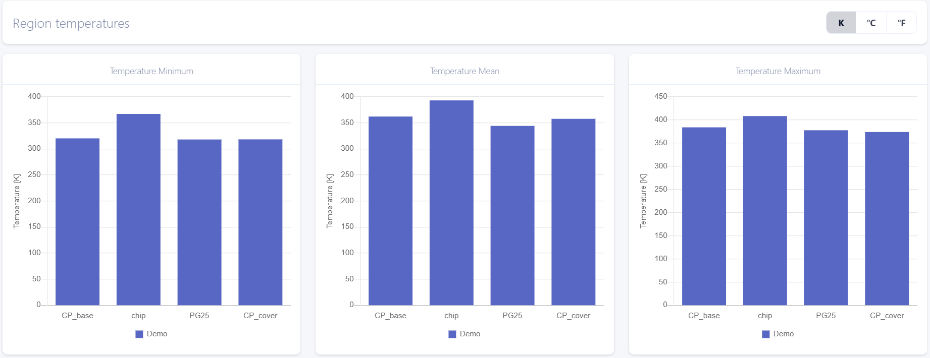
Bar Chart example
3D results
When a full CFD resolution is executed, the 3D Results section provides an interactive graphical interface for spatial data analysis. This visualization environment allows for a comprehensive inspection of the thermal and fluid behavior directly mapped onto the generated geometry.
The interface includes a robust set of post-processing tools:
- Mesh Visualization: Inspect the underlying computational grid used for the simulation.
- Surface Plots: Evaluate temperature, pressure, or velocity distributions on the exterior faces of solid bodies and fluid boundaries.
- Streamlines: Generate and track fluid flow paths to identify recirculation zones, bottlenecks, or flow distribution patterns.
- Cross-Sectional Slices: Probe internal fields by placing arbitrary clipping planes through the domain to visualize internal gradients.
| Region | Subregion | Boundary | |||
|---|---|---|---|---|---|
| Solid | Fluid | Design | General | All types | |
| Visualization Types |
|
|
|
|
|
| Fields | , aspectRatio, nonOrthogonalityAngle, skewness | , aspectRatio, nonOrthogonalityAngle, skewness | , aspectRatio, nonOrthogonalityAngle, skewness | Same as parent region | Same as parent region |
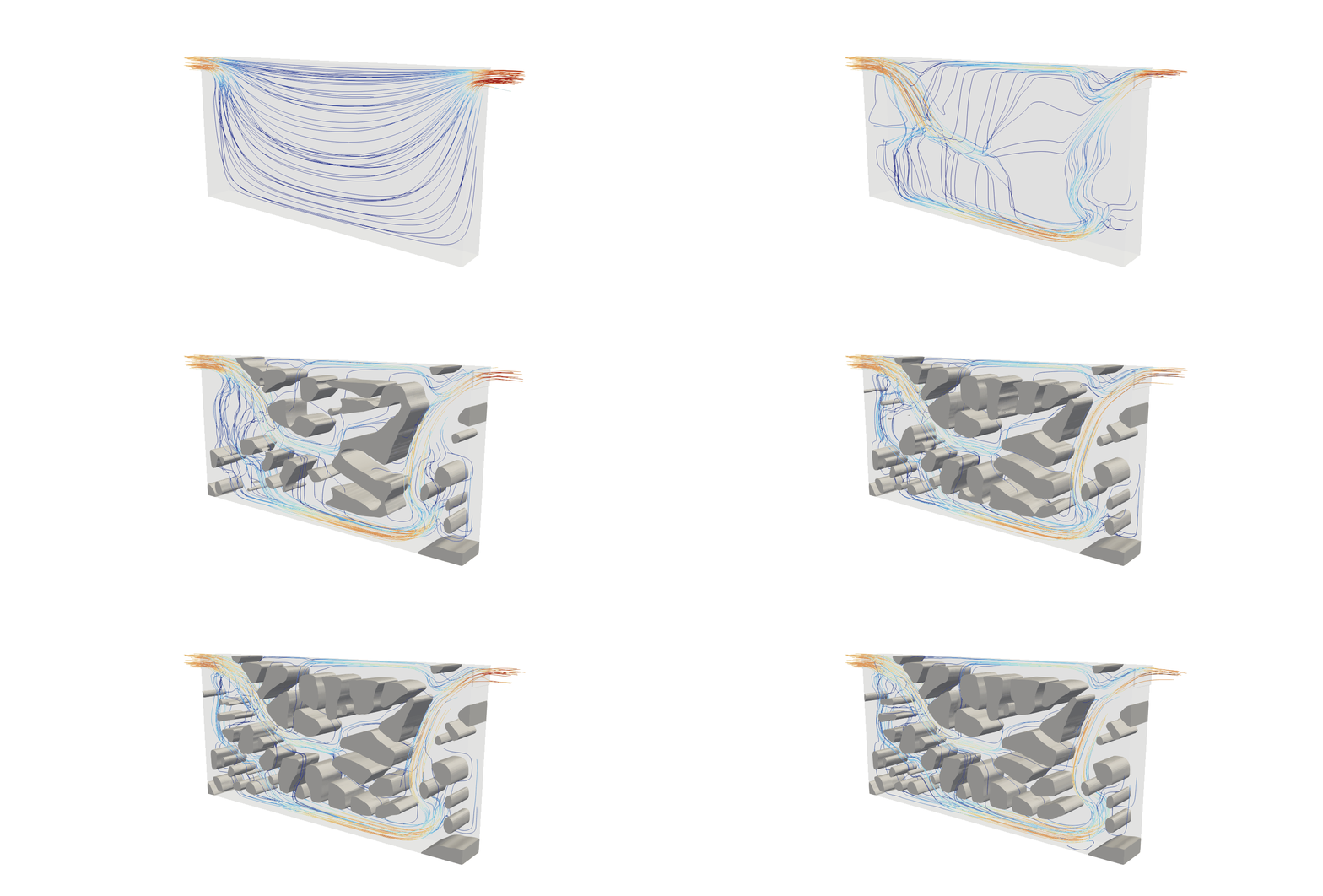
Streamline evolution for a case while the case is being optimized.
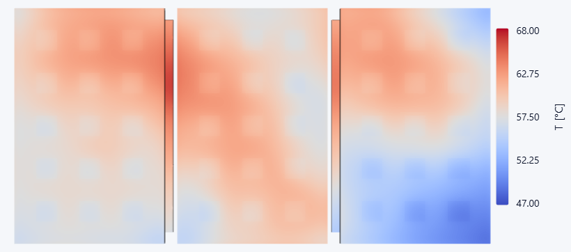
Temperature surface plot of a heat source after optimization.
Configuration tools
View manipulation
The mouse and keyboard shortcuts to manipulate the view are listed in the table below.
| Action | Binding |
|---|---|
| Rotate | Left mouse button |
| Zoom | Right mouse button/mouse wheel |
| Pan | Shift + left mouse button |
The view can also be manipulated using the buttons on the 3D view. There are options to take screenshots, change camera angles, and orient the view in the X, Y, or Z axis.
Plot manipulation
To view the options for each plot, click on the plot such that the name turns bold. Now a side pane appears on the right side of the window where you can select the field, color scheme, or value ranges for the plot. To hide/show a particular plot, use the icon on the left side of the name of the plot.
Updated 27 days ago