Physics

Introduction

This page details which physical phenomena are included and how you as a user can influence them. Please navigate to the phenomenon you are interested in to learn more about it.

Heat sources

Introduction

A source is where heat enters your case. On ColdStream there are two types of sources: indirect sources and direct sources. Direct sources are controlled by the user during the case setup. A user can specify this heat input during the case setup. On the other hand, indirect sources are unaffected by the user during the case setup. For example, viscous dissipation in the fluid region(s) will always be activated when a case is running.

This article focuses solely on how you can correctly use direct sources on ColdStream.

	User input	Unaffected by user
Direct source	Yes
Indirect source		Yes

What are direct sources

Direct sources are heat inputs specified directly by the user during the case setup. These sources are due to Joule heating, chemical reactions, or some other phenomenon.

This quantity of heat is spread out evenly over the entity on which it is defined, meaning that:

• if the heat input $(\dot Q)$ is specified on a surface patch: the local heat map $(q \;\text{in}\left[ \frac W{m²} \right])$ is uniform:

  $$q=\frac{\dot Q}A$$

  Where $A$ is the area of the surface patch.

• if the heat input $(\dot Q)$ is specified on a (sub)region: the volumetric heat map $(q \;\text{in} \left[\frac W{m^3}\right])$ is uniform:

  $$q=\frac{\dot Q}V$$

  Where $V$ is the volume of the (sub)region.

If the input value is negative, the heat source becomes a heat sink. This means that instead of heat entering through that entity, it leaves through that entity.

❗️

Important

The specified quantity of heat is spread out uniformly over the entity on which it is defined.

How to use direct sources?

As stated earlier, direct sources are specified by the user during the case setup. A user has the choice to include a heat source for all entities (regions, subregions, and surface patches) available in the geometry. The following subsections go into more depth on how to assign these heat sources for each of the entities individually.

Direct sources on regions and subregions

During the case setup, all regions (not including the subregions) have an input field for a heat source (Q). By default it is set to 0, meaning no heat is entering or leaving through it. Fill in the required value if you want to overwrite that default value.

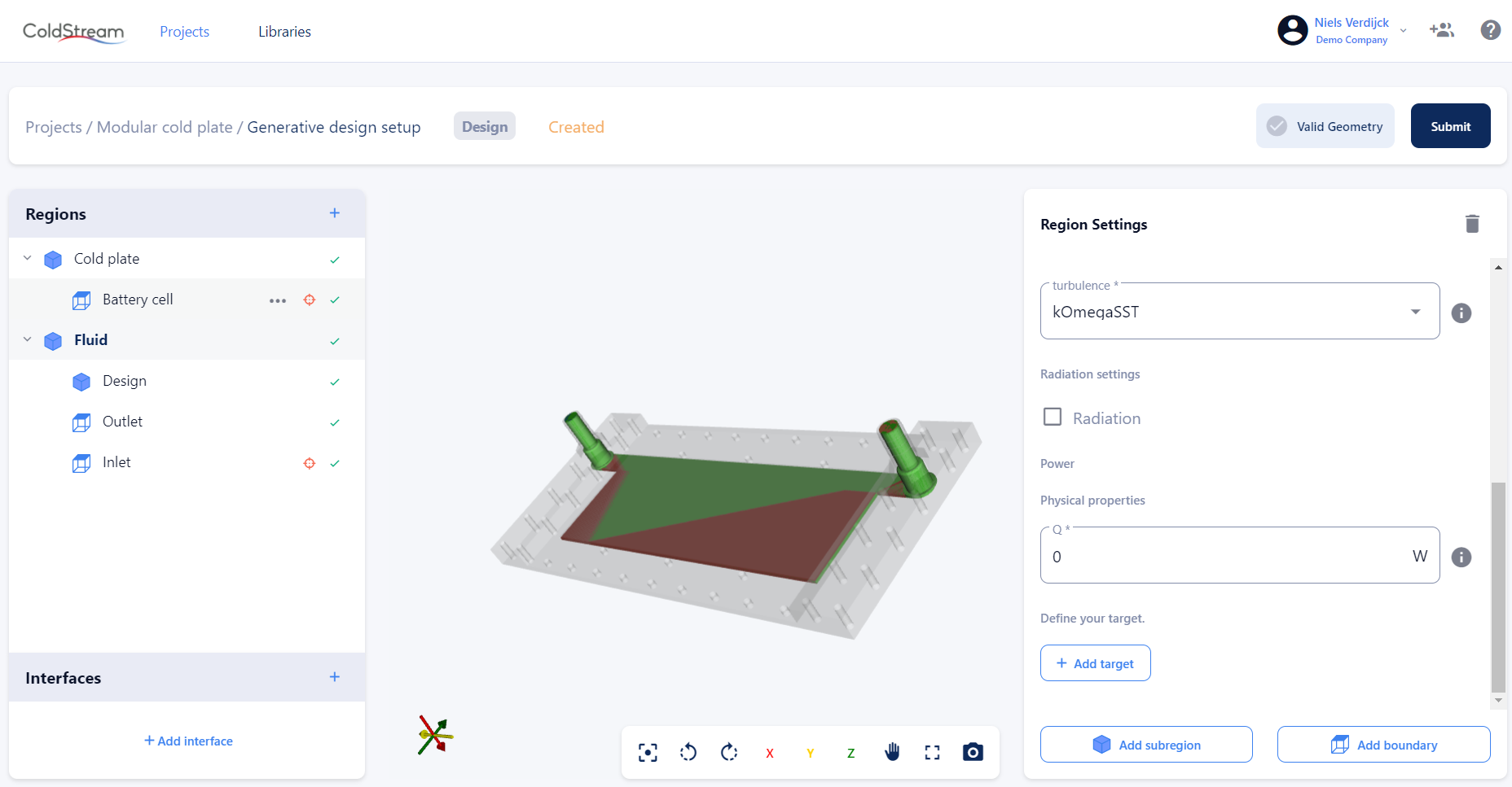
Heat source input field for a region

As stated in the previous section, the inputted value is distributed uniformly over the entire volume. In case you want a more localized heat production, you can include a subregion. This subregion must be of type 'general', not of type 'design'.
The heat source input field is identical to the one of a parent region. However, the heat is now distributed uniformly in that subregion only, not in the entire parent region. You can include as many subregions as you like, as long as they don't overlap. Be warned though, that the more regions you include, the longer it will take for the platform to complete your case.

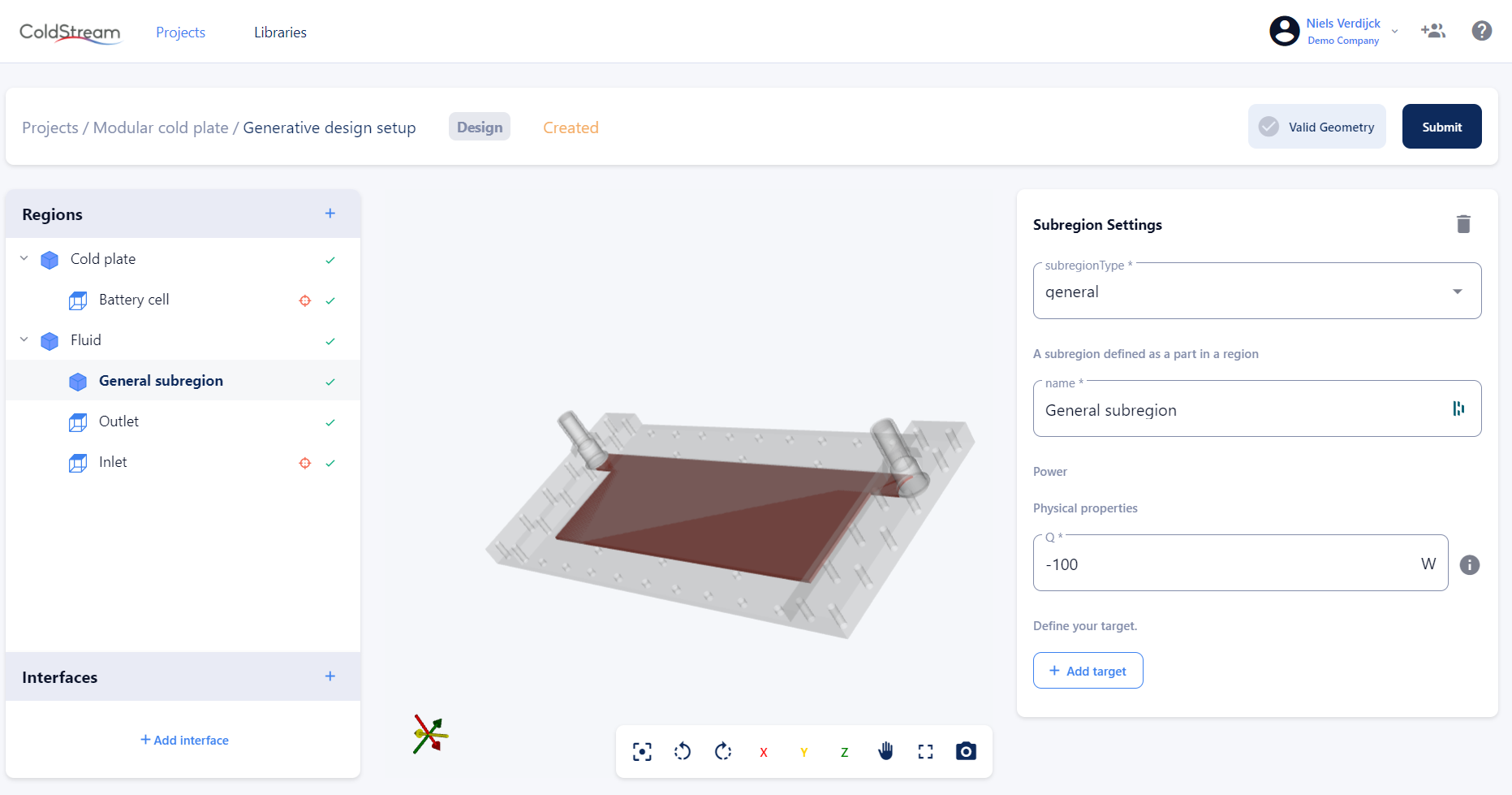
Heat source input field for subregions of type 'general'

Direct sources on surface patches

There are only two types of surface boundary conditions that allow you to specify a direct heat source. These are the heatedWall boundary condition and the insulatedWall boundary condition.

The heatedWall boundary has the same heat source input field as the regions and subregions have. The inputted value will be distributed uniformly over the entire area of this surface patch.

An insulatedWall does not allow any heat to be transferred through it. This means that you explicitly tell ColdStream that heat can't enter or leave this surface patch. An insulatedWall is also assumed wherever a region does not have an interface with another region.

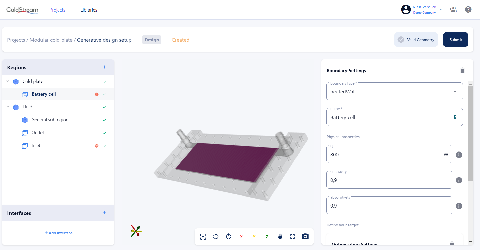
Heat source input field for heatedWall boundary

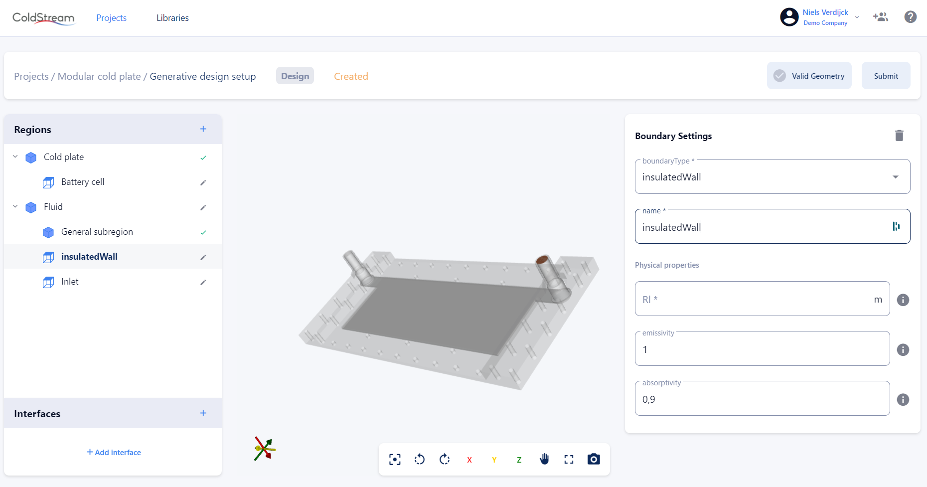
Input settings for an insulatedWall boundary

📘

Note

Subregions of type 'general' and surface patches of type 'heatedWall' allow you to specify a localized heat input for your case.

---

Radiation

Introduction

For bodies with varying temperatures, the energy exchange can occur in three modes: conduction, convection, and radiation. Conduction is the heat transfer by direct contact, convection is the heat transfer by motion of a material and radiation is the transfer of energy with the help of electromagnetic waves. In this article, we take a deeper look into the radiative heat transfer.

Electromagnetic radiation is emitted by heated surfaces. This means all materials with an absolute temperature above zero degrees Kelvin, radiate thermal energy. The hotter the object, the more it will radiate to its colder surroundings, and the more important it becomes to take radiative heat transfer into account in your simulations. Radiation distinguishes itself from conduction and convection as it does not necessarily need a medium to carry it. Radiation can thus occur through any transparent medium, either a fluid, a solid, or a vacuum.

In radiative heat transfer, the Stefan-Boltzmann law is a well-known formula as it relates the heat flow rate emitted or absorbed from an object to the fourth power of its absolute surface temperature.

$$q_r=\epsilon\sigma T^4A$$

In the formula above, $\epsilon$ represents the emissivity, $\sigma$ the Stefan-Boltzmann constant, $T$ the temperature expressed in Kelvin $[K]$ and $A$ the surface of the emitting body.

Besides the temperature of the surface, the rate at which a body radiates thermal radiation also depends on the surface properties. A surface with an emissivity of one is called a black body. This black body is an idealized object that would absorb all wavelengths of thermal radiation it would receive, without reflecting or transmitting any energy. Hence, it would absorb light and appear black at low temperatures. However, black bodies don’t exist in real life, in reality, all objects are gray bodies. This means incident radiation on a surface is partly reflected, absorbed, and transmitted according to the surface properties. For gray surfaces, the following condition holds:

$$\epsilon + \tau +\rho = 1$$

Where $\epsilon$ denotes the emissivity, $\tau$ the transmissivity and $\rho$ the reflectivity of the surface.

Furthermore, Kirchoff discovered that a good emitter is also a good absorber so the emissivity $(\epsilon)$ of a surface can be linked to the absorptivity of a surface $(\alpha)$ as follows:

$$\epsilon=\alpha$$

If a medium absorbs, emits, or scatters a thermal ray as it passes through, it is called a participating medium. The ray can lose energy through absorption and scattering away from the ray. However, energy can also be gained from light sources in the medium through emission and scattering towards the ray. If the medium does not absorb, emit, or scatter a thermal ray, the medium is called a non-participating medium.

The energy balance of the ray over an infinite layer of the medium, results in a differential equation, i.e. the radiative heat transfer equation (RTE). Within our software, the RTE is solved with the Finite Volume Discrete Ordinates Method or FvDOM model in short. This means the RTE is solved for a discrete number of finite solid angles. This model is the most comprehensive radiation model, which can be used for (semi-) transparent media and can account for scattering and wavelength-dependent transmission. Our model can handle both participating and non-participating media. In the first case, the RTE is coupled with the general energy equation for fluids or solids, and a source term is added to the energy equation to account for the radiative heat transfer, in the latter the source term is zero.

When to enable radiation?

If large temperature differences are to be expected concerning the surroundings, radiative heat transfer will become important as it relates to the fourth power of the temperature. In this case, radiation should be enabled. When the radiative heat transfer is expected to be small with regards to the convective heat transfer, radiation should not be enabled; unless this specifically needs to be modeled.

Which parameters to set in the platform?

📘

How to enable radiation?

1. Enable radiation in the concerned region by checking the radiation checkbox in the region settings window.
2. In the boundaries related to the region, fill in the emissivity and absorptivity parameters in the boundary settings window.
3. If the region is a solid type, fill in the absorption coefficient in the solid material properties.

When radiative heat transfer is to be included in a specific region and the medium of the region is considered to be participating, (i.e. the medium absorbs, emits, or scatters a thermal ray as it passes through) needs to enable radiation in the concerning region by checking the radiation box. In addition, the following parameters need to be set in the boundary settings of the boundaries related to the concerning region. If the concerning region is a solid type, also some material parameters related to radiation can be set:

Parameter	Units	Explanation
Boundary settings
$\varepsilon$	$[-]$	The emissivity of the boundary. This is a dimensionless value between 0 and 1. If no value is specified, a default value of 0.9 is adopted.
$\alpha$	$[-]$	The emissivity of the boundary. This is a dimensionless value between 0 and 1. If no value is specified, a default value of 0.9 is adopted.
Solid material parameter setings
$absorption$	$[1/m]$	The absorption coefficient represents the attenuation of the radiation intensity.

On the boundaries, emissivity and absorptivity should be specified. The emissivity depends on the material of the surface and measures the capability to emit radiation. It is a representation of the ratio of energy radiated by the material to the energy radiated by a black body at the same temperature. The emissivity is considered constant for every material. In reality, the emissivity depends on the wavelength of the radiation that is being emitted. However, in CFD, the total emissivity is specified which is an integrated emissivity over all wavelengths. The emissivity of a surface is bound between 0 and 1. A perfect mirror, for example, would reflect all energy, hence the emissivity, and by Kirchhoff’s law, the absorptivity is zero. Within our software, the default value is set to 0.9.

The absorptivity is a dimensionless value between 0 and 1. If nothing is specified, the same value as the emissivity is taken by default.

When dealing with participating media in the simulation, some additional parameters need to be set. Since part of the radiative heat transfer can be absorbed in this case, leading to a change in radiation intensity, an absorption length should also be specified which represents the attenuation of the radiation intensity.

---

Turbulence

Introduction

In fluid dynamics, flow can either be considered laminar or turbulent. In the first case, the fluid particles follow a smooth path with almost no mixing or disruption between adjacent paths. On the other hand, in turbulent flow, the flow becomes very irregular and the fluid particles follow a chaotic path, full of eddies, swirls, and flow instabilities.

Turbulent flows are common in real life, think for example of the blood flow in your veins, the airflow over the wing of a plane, and breaking waves at the beach, ….

In the 19th century, Reynolds was one of the first scientists to perform a set of experiments and show the transition between laminar and turbulent flow regimes and link this transition to the ratio of the inertial and the viscous forces.

$$Re=\frac{inertia\;forces}{viscous\;forces}=\frac{\rho\cdot u\cdot l}{\mu}$$

With $\rho$ the density of the fluid, $u$ the velocity of the flow, $l$ a characteristic length scale and $\mu$ the viscosity of the fluid.

This Reynolds number is still widely used today to characterize flow regimes. When the Reynolds number is smaller than 2300 in circular tubes, a laminar flow regime will occur. If the Reynolds number is higher than 4000, the flow will be turbulent. Everything in between is called the transitional regime.

When running simulations with turbulent flow, the turbulence needs to be resolved or an appropriate model needs to be selected. Turbulence models are simplified constitutive equations that predict the evolution of the turbulent flow. Even though a lot of research has been done over the past decades, turbulence modeling is still not a trivial task.

The difference between DNS, LES, RANS

Three main approaches can be distinguished: DNS, LES, and RANS to predict the evolution of the turbulent flow.

DNS

Turbulence can be fully described and resolved by the complete unsteady Navier-Stokes equations without the use of any modeling assumption regarding turbulence. This is called DNS, which means a Direct Numerical Simulation is performed. However, this requires extreme computational resources as the mesh resolution and the time steps need to be extremely small to capture the full range of temporal and spatial scales. This makes the DNS approach impractical in industrial applications and is mainly considered as a research tool.

LES

In the Large Eddy Simulation approach, or LES in short, the most energy-containing structures of the flow, i.e. the large eddies are still resolved. Smaller scales of turbulence are treated by turbulence models instead.

RANS

The RANS, or the Reynolds-Averaged Navier-Stokes approach is the most commonly used approach in industrial applications. In most engineering applications, we are only interested in mean or integral quantities and to obtain these, solving turbulent flow with a turbulent model is the most cost-effective way and sufficient to obtain good results. In this approach, the Navier-Stokes equations are averaged to obtain the mean equations of the fluid flow. These averaged equations are similar to the full Navier-Stokes equations but contain some additional terms in the momentum equations called the Reynolds stresses due to the nonlinearity of the equations. These Reynolds stresses are unknown and need to be modeled with a turbulence model.

There are a lot of different RANS models available, only the most commonly used are elaborated on in more detail. Each of these models has its limitations due to the specific modeling assumptions.

$k-\epsilon$ model

The $k-\epsilon$ model is a two equation model. This means that in addition to the conservation equations, two additional transport equations are solved. One for the turbulent kinetic energy $k$ which determines the energy in the turbulence and $\epsilon$ one for which represents the turbulent dissipation. The $k-\epsilon$ model also requires wall functions to obtain a value of near the wall. The $k-\epsilon$ model has proven to provide reliable results for flows with relatively small pressure gradients. When a problem involves large adverse pressure gradients, large separations or complex flows with strong curvatures, the $k-\epsilon$ model is not the most suitable turbulence model. A lot of different variations exist of the $k-\epsilon$ model, a few examples are the RNG $k-\epsilon$ model or the LaunderSharma $k-\epsilon$ model. All of these variations have their modifications to perform better under specific conditions.

RNG $k-\epsilon$ model

The RNG $k-\epsilon$ model was developed using the Re-Normalization Group (RNG) methods by Yakhot [1] to renormalize the Navier-Stokes equations to account for smaller scales of motions. This model is more suitable than the standard $k-\epsilon$ model for swirling flows, separation or shear flows. It is also known to underestimate the value of the turbulent kinetic energy and thus creating a less viscous and more realistic flow with complex geometries. It is however not as widely used as the standard $k-\epsilon$ model.

LaunderSharma $k-\epsilon$ model

The LaunderSharma $k-\epsilon$ model [2] is a low-Reynolds $k-\epsilon$ model for incompressible, compressible and combusting flows including a rapid distortion theory (RDT) based compression term.

$k-\omega$ model

The $k-\omega$ is also a two equation model, meaning two additional transport equations are solved. One for the turbulent kinetic energy $k$ and one for the specific turbulent dissipation rate $\omega$. The model used in the software, is based on the formulation by Wilcox [3]. $k-\omega$ models are also commonly used. The standard formulation is a low Reynolds model, which means it can be used for flows with low Reynolds numbers where the boundary layer is relatively thick and the viscous sublayer can be resolved, without the need for wall functions. The $k-\omega$ has shown to perform better in complex boundary layer flows under adverse pressure gradients and separations with respect to the $k-\omega$ models. However this model is also known to overpredict separation or shear stresses of adverse pressure gradient boundary layers and is known to be sensitive to inlet free stream turbulence properties.

$k-\omega$ SST model

The $k-\omega$ SST model is also a popular choice. This model, developed by Menter [4], employs a shear stress transport (SST) formulation which combines the $k-\omega$ and the $k-\epsilon$ model . In the outer region and in the outside of the boundary layer, the $k-\epsilon$ model is used. In the inner boundary layer, the $k-\omega$ model is used. By combining the two models, the disadvantages of both models are eliminated. The $k-\omega$ SST model model can be used all the way down to the wall and the sensitivity to the inlet free stream turbulence is eliminated by using the $k-\epsilon$ model in the outer region.

Which model to choose in your application?

The selection of the turbulence model is important. Based on our experience, we can make the following recommendations.

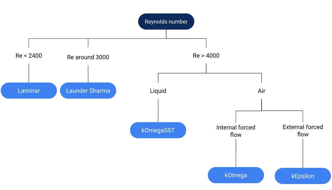
Turbulence model selection chart

First, the Reynolds number of the flow should be estimated. This Reynolds number just needs to be estimated to determine whether or not your case is turbulent. It is acceptable to make assumptions and simplifications regarding the geometry or parameters.

Let’s for example calculate the Reynolds number for water flowing through a pipe with a diameter $d$ of 1.0 m and a speed of 1.5 m/s. In case you have a pipe or duct, the characteristic length scale in the Reynolds formula is equal to the hydraulic diameter, which can be calculated as follows, with $A$ the area section of the duct or pipe in $[m^2]$, $P$ the perimeter of the duct or pipe in $[m]$:

$$l=d_h=\frac{4A}{P}=\frac{4(\pi d^2/4)}{\pi d}=d$$

So for a simple pipe or tube, the hydraulic diameter is equal to the diameter of the duct or pipe. So filling in the Reynolds equation as described before, gives:

$$Re=\frac{(1000\frac{kg}{m^3})(1.5\frac ms)(1m)}{0.00959\frac{kg}{m\cdot s}}=156\;413$$

From which can be determined, the flow can be considered turbulent. If you don’t know what the Reynolds number would be for your case and find it difficult to calculate, it is probably turbulent (Re>4000). If you have a case with very small parallel channels and a low velocity, chances are high that your case will be laminar.

With the Reynolds number determined, an appropriate turbulence model can be selected. If this Reynolds number is very low (Re < 2400) a laminar model should be selected.

If you expect your flow to be in the transitional regime, i.e. a Reynolds number around 3000, the best choice according to our experience is the LaunderSharma model as this model is appropriate for low Reynolds simulations.

If turbulent flow is to be expected and you are simulating a liquid flow, the $k-\omega$ SST model should be selected. In the case of air flow, $k-\omega$ model is the best model for internal forced air flow in our opinion. For the case of external forced air flow, the $k-\epsilon$ model should be selected.

Still in doubt about which model to choose after reading this? We suggest you take the $k-\omega$ SST model as a starting point and see if the obtained results match your expectations.

References

1. V. Yakhot, S.A. Orszag, S. Thangam, and C.G. Speziale. Development of Turbulence Models for Shear Flows by a Double Expansion technique. Physics of Fluids A Fluid Dynamics, 4(7), 1992.
2. B.E. Launder and B.I. Sharma. Application of the energy-dissipation model of turbulence to the calculation of flow near a spinning disc. Letters in heat and mass transfer, 1(2), 131-137, 1974.
3. D.C. Wilcox. Turbulence modelling for CFD, 2, 103-217. 1998.
4. F.R. Menter and T. Esch. Elements of Industrial Heat Transfer Prediction. 16th Brazilian Congress of Mechanical Engineering (COBEM), 2001.

---

Buoyancy

Introduction

The definition says it is an upward directed force, exerted by a fluid, that opposes the weight of the partially or fully immersed object and was first described by Archimedes more than 2000 years ago.

So let’s take a look at an example and assume we have a cylindrical object, completely submerged in a box of water. The water pressure increases linearly with the depth, so the water pressure at the bottom of the cylinder is larger than the water pressure at the top of the cylinder.

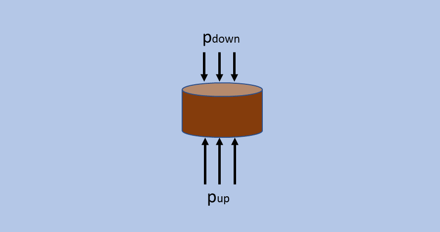
Buoyancy schematic

If we express this in terms of forces, we can say that the pressure difference will result in a net upward-directed force on the cylinder, which is called the buoyant force.

$$F_{buoyant}=F_{up}-F_{down}$$

By taking into account the following relation between pressure and forces, $F=\rho\cdot A$, the equation above can be rewritten as:

$$F_{buoyant}=p_{up}A-p_{down}A=(p_{up}-p_{down})A$$

And taken into account that the pressure can be expressed as $p=\rho gh$, the buoyant force can be written as:

$$F_{buoyant}=\rho_fg(h_{top}-h_{bottom})A$$

with $h_{top}$ and $h_{bottom}$the depths of the top and bottom of the cylinder respectively and $\rho_f$ the density of the fluid.

The term $(h_{top}-h_{bottom})\cdot A$ can also be written as a volume. This is the volume of displaced fluid by the submerged object and not the volume of the object itself. When an object is fully submerged, both volumes are equal. However, when an object is only partly submerged the volume of the displaced fluid is smaller than the volume of the object and only the submerged volume should be taken into account.

So the final equation becomes:

$$F_{buoyant}=\rho_fgV_{displaced\;fluid}$$

Hence the buoyancy force depends on the density of the fluid in which it is submerged, the gravity, and the volume of displaced fluid. This force is independent of the mass or the density of the submerged object. Furthermore, this force is also independent of how deep the object is in the fluid as the pressure at the top and the bottom of the object increases by the same amount if you go deeper.

On every object, fully or partially submerged, there will be a buoyant force upwards. However, depending on the weight of the object $(F_g)$ it can either:

• Sink when $F_g > F_{buoyant}$

• Remain in place when $F_g=F_{buoyant}$

• Rise upwards when $F_g < F_{buoyant}$ and the object is fully submerged or floats when the object is only partially submerged.

An important example of when buoyancy is important is in natural convection cases, as in such cases the fluid motion occurs by buoyancy effects. When a heat source is added to the fluid, the density will vary with the temperature. The material will become less dense with increasing temperature and cause the hot fluid to rise. Buoyancy is also present in forced convection cases but is less dominant.

How buoyancy is taken into account in the platform

When the density variation is limited, the density can be taken as a constant in the unsteady and convection terms and only as a variable in the gravitational term. This method, the so-called Boussinesq approximation, is implemented in our platform to account for buoyancy. The density which takes into account the thermal expansion is calculated as:

$$\rho_{eff}=\rho(1-\beta(T-T_{ref}))$$

With $\rho_{eff}$ the effective driving density, $\rho$ the density, $T$the temperature, $T_{ref}$ the reference temperature and $\beta$ the thermal expansion coefficient.

Note that the effect of buoyancy on turbulence is also taken into account in our platform. This happens fully automatically through the application of source terms on the turbulent kinetic energy $k$ and the turbulent kinetic energy dissipation rate $\varepsilon$ or specific dissipation rate $\omega$ depending on the chosen turbulence model.

Which parameter to set in the platform

When buoyancy effects are to be included in a specific region, several parameters need to be set. These parameters are set in the region settings of the concerned region:

Parameter	Units	Explanation
$g$	$[m^2/s]$	The directional gravity vector.
$\beta$	$[1/K]$	The thermal expansion coefficient needs to be set for the material that is assigned to the region. It can be specified as a constant value or an array with the polynomial coefficients to include the temperature dependency.
$T_{ref}$	$[K]$	Optional: The initial temperature in the specific region, serving as a reference temperature. If nothing is specified, a temperature of 293.15 $K$ is set.
$p_{ref}$	$[Pa]$	Optional: The initial pressure in the specific region, serving as a reference pressure. If nothing is specified, a pressure of 1 $atm$ (101325 $Pa$) is set.

---

Rotation

Introduction

Rotation occurs in various engineering applications, such as turbomachinery (e.g. pumps, fans, turbines), rotating machinery (e.g., mixers, agitators), and automotive systems (e.g. wheels, gears). Understanding the flow dynamics around rotating components is crucial for optimizing performance, improving efficiency, and ensuring reliable operation.

In computational fluid dynamics (CFD) simulations, incorporating rotation can significantly enhance the accuracy and realism of the results, especially in scenarios involving rotating components. Rotation introduces complexities that must be appropriately accounted for in the simulation setup to ensure accurate predictions of flow behavior and heat transfer. This way, engineers can gain valuable insights into the effects of rotational motion on flow patterns, pressure distributions, and heat transfer phenomena.

How rotation is taken into account in ColdStream

In ColdStream, rotation is implemented using the Multiple Reference Frame (MRF) method. This method is a widely used approach for simulating flow around rotating components in CFD software. This method simplifies the computational domain by dividing it into stationary and rotating regions, allowing for efficient numerical solutions without explicitly resolving the motion of each rotating component.

In the MRF model, the computational domain is divided into multiple reference frames, each associated with a specific rotational speed and axis of rotation. The key principle behind the MRF method is to transform the governing equations from the absolute frame of reference to the relative frames, where the effects of rotation are accounted for through additional source terms in the momentum and energy equations. These source terms represent the centrifugal and Coriolis forces induced by rotation, enabling accurate prediction of flow behavior around rotating components.

📘

Note

The MRF method is used in ColdStream to model rotation. This method divides the computational domain into multiple reference frames.

❗️

Important

The division of the computational domain into multiple reference frames is performed automatically by ColdStream in the background. There is no need to prepare an MRF zone in your CAD model.

Which parameters to set in ColdStream?

In the platform, the convention is to specify solid regions as rotating, and fluid regions as stationary. To enable rotation for a specific (solid) region, first click the “Add rotation” button in the “Region Settings”.

Then, you can specify the remaining inputs:

• The rotation axis direction: around which axis is the component rotating? (X, Y, or Z in the principal axis system
• The rotational velocity: how fast is the component rotating? [rad/s]

❗️

Important

Rotation should be enabled for each rotating region separately. Take care to ensure that the rotating region(s) are (predominantly) axisymmetric and will not intersect or overlap with other (solid) regions when they are rotated around their center of rotation.

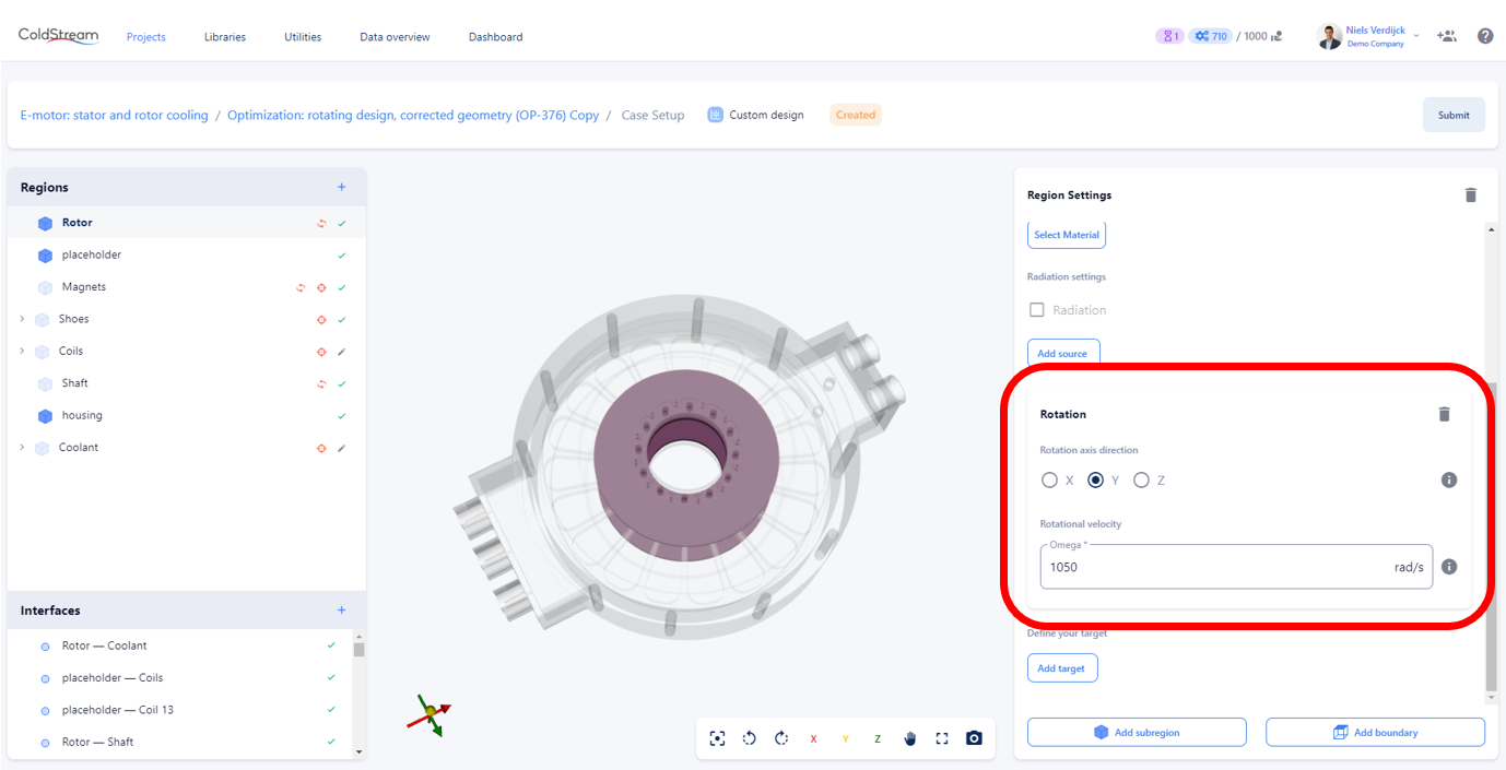
Input fields for rotation