Thermal network

Introduction

All CFD thermal engineers would like their simulations to be as accurate as possible while also running as fast as possible. This of course leads to a contradiction, as increasing the accuracy of a simulation requires it to capture more details and thus to run for a longer time. This is why a trade-off cannot be avoided and typical CFD simulations can run for multiple hours or even days (for very complex cases) on ColdStream.

However, there are ways to simplify the complexity of a simulation to get results in a matter of minutes. The thermal network approach is one such way.

Thermal network estimation

Once your case is fully set up on ColdStream and is ready to be submitted for simulation or standard design, you can submit it as a 'Correlation based estimation'. Then, a thermal network representing your case will be constructed and simulated.
In the case of a standard design, a thermal network will be generated for each heat sink type that is tested.
Lastly, if you submit a case of type 'Simulation', a thermal network will be generated before beginning the CFD computation, giving you a quick first impression of the thermal behavior of the case in question.

The estimation will use correlation-based techniques to be able to provide rough estimates of the thermal resistance values at each connection between two regions or between a region and a boundary. Given these thermal resistances, the expected temperatures and heat fluxes can be derived using integrated equations, so in a computationally cheap way.
This option requires only 1 credit and its results are delivered within an hour at most, thus making it a very interesting trade-off between accuracy and resources spent.

Once you get notified about your thermal network being published, you can click on the 'Thermal network'-tab and you will see a diagram similar to the figure below. In the case of a standard design, a new corresponding thermal network is displayed every time you select an iteration number.

Thermal network example

Diagram features

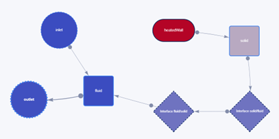
The thermal network contains different symbols, the following list explains what each symbol represents:

• Solid squares correspond to regions.
• Solid ovals correspond to thermal boundaries.
• Dashed diamonds correspond to interfaces between two adjacent regions. There will always be two diamond symbols next to each other (representing the Region1-Region2 interface as well as the Region2-Region1 interface).
• Dashed circles correspond to fluid boundaries.

The box representing the entity with the highest (respectively lowest) temperature is colored in dark red (respectively dark blue), and all temperatures in between get assigned intermediate shades of red or blue.

Each box is connected to at least one other box with a directed arrow. These arrows indicate the direction of the heat flow, showing in the blink of an eye the general thermal path that will result from your case setup. For fluid boundaries, the arrows will always point from the inlet(s) toward to fluid region(s) and then onwards to the outlet(s).

By hovering over a box, a pop-up window appears displaying the estimated mean temperature of the corresponding region in a steady state regime. Keep in mind that this is a rough estimation and can deviate somewhat from the temperatures that would come out of the full CFD analysis.
You can also look at the estimated velocities, pressures, and mass flow rates (if applicable to the entity of interest). Lastly, ColdStream will also display the estimated heat flux and thermal resistance values when hovering over the arrows connecting each of the diagram features.

📘

Note

Note that you can drag the whole thermal network or independent boxes and zoom in or out, leaving you the freedom to display the boxes most optimally for your convenience. This is especially useful if your case contains a lot of entities.

Thermal network after CFD analysis

Although the thermal path and the connections between regions are already exact in the estimation mode, if you want to know the exact values of the temperatures or thermal resistances themselves, you need to submit a full CFD simulation. At the end of your simulation, you will see a new thermal network diagram displayed with updated values. The mean temperatures, heat fluxes, and resistance values now come directly from a fully converged CFD simulation rather than being estimated based on correlations.
One can still manipulate the diagram in the same way as was explained in the 'Note'-box above.

How to use thermal networks efficiently

To close this article, we'll use a simple example case to showcase the usefulness of the thermal network feature. For this example, we'll use two boxes ('Box1' and 'Box2' respectively) that touch each other. 'Box1' is heated on one side by a boundary condition called 'Wall1', while one boundary of 'Box2' is kept at a constant temperature of 20°C (293.15 K) by 'Wall2'. All free-floating edges of both regions are insulated.

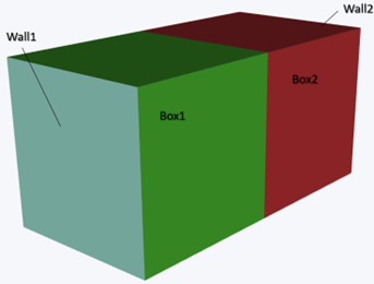
Example geometry

In a steady state regime, the heat will flow from 'Wall1' to 'Wall2'. This means that the case can be simplified to the following network.

Thermal network for example geometry

Suppose that you do not have any specification about the amount of heat entering through 'Wall1' and that you want to know what power as a boundary condition would lead to a mean temperature close to 303.15K inside 'Box1'. Rather than running a bunch of simulations with varying power values, you should consider running a first thermal network estimation with arbitrary power and see the resulting temperature.

Let us perform this with a heat input of five Watt $(\dot Q=5W)$. From the correlation based estimation, this will result in the following mean temperature for 'Box1':

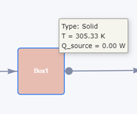
Mean temperature 'Box1'

You can see immediately that the heat input is too high and that 'Box1' is expected to exceed the desired mean temperature. Next, a second attempt with an input of Q = 3W leads to an estimation of 300.46K for the mean temperature, which is too low. However, you now know that 'Wall1' should be heated with a total power of around Q = 4W to result in a mean temperature of 'Box1' close to 303.15K! You can now finally submit your simulation with that desired heat input.

📘

Note

The more complex your setup, the more difficult it becomes for the estimation to remain close to the actual temperature value. But you can see now how you can use the ‘quick estimation’ mode to get valuable information for free and in a limited amount of time.