Targets and weighting functions

Introduction

When all geometrical entities are uploaded, the physics and boundary conditions are set, and the design volume is defined, are you able to dictate what ColdStream needs to optimize. This can be defined through targets. ColdStream also gives its users control over the priority of these targets through weighting functions.

Targets

Introduction

To create a design, one or multiple design targets should be set. A target is a goal that the design process of a component should aim to meet. A design problem can have a single or multiple targets. For multiple target problems, these are often not complementary, therefore in practice, a design will mostly incorporate tradeoffs. To better manage those trade-offs, targets can be of one of two types: an objective or a constraint.
The following article goes into more detail about how changing the weighting values impacts the optimized designs.

To better manage those trade-offs, targets can be of one of two types: (1) an objective or (2) a constraint.

❗️

Important

A design objective is a target or goal which is minimized or maximized. It is a target which is aimed to have “as little as possible” or “as much as possible”. An example goal could be maximal cooling efficiency.
A design constraint is a target which has to be satisfied, in terms of “less than X” or “more than Y”. An example could be weight, or the required pumping power being lower than the available one.

📘

Note

A target should be measurable and should be rigorously defined. A target is set on an entity (region, subregion, boundary). Every target or every combination of targets can lead to a unique output.

	Region		Sub region		Boundary
					Inlet				Outlet			Wall
	Solid	Fluid	Design	General	FixedFlowRateInlet	PressureInlet	FanInlet	PumpInlet	PressureOutlet	FanOutlet	PumpOutlet	HeatedWall	ExternalWall	FixedTemperatureWall	InsulatedWall
Objectives
PowerDissipationMinimization
PressureLossMinimization
RelativeVolumeMinimization
RelativeVolumeMaximization
TemperatureMinimization
TemperatureSpreadMinimization
TemperatureVarianceMinimization
VelocityVarianceMinimization
VelocitySpreadMinimization
ElectricWirePowerMinimization
Constraints
PowerDissipation
PressureLoss
MinimumRelativeVolume
MaximumRelativeVolume
MinimumTemperature
MeanTemperature
MaximumTemperature
TemperatureVariance
VelocityVariance
MaximumElectricWirePower
MaximumHeatingTime

Objectives

1. PowerDissipationMinimization
2. PressureLossMinimization
3. RelativeVolumeMinimization
4. RelativeVolumeMaximization
5. TemperatureMinimization
6. TemperatureSpreadMinimization
7. TemperatureVarianceMinimization
8. VelocityVarianceMinimization
9. VelocitySpreadMinimization
10. ElectricWirePowerMinimization

PowerDissipationMinimization

Name	PowerDissipationMinimization
Goal	Minimize the Power Dissipation of the flow through the design.
Applicable to	Region	Fluid
	Subregion	Not applicable to any subregion types
	Boundary	Not applicable to any boundary types

Use this goal function if you want to reduce the viscous and pressure losses of the flow through the design. This is of special importance on complex systems, where the fluid flows through several components, each with specific optimal operating conditions that need to be met. Furthermore, if the flow is driven by pumps or fans, minimizing the power dissipation results in a general improvement of efficiency. The power losses in the flow are usually related to recirculation bubbles, turbulence and sudden changes in the flow velocity, so by using this objective, the flow should become more uniform. In other words, the fluid will flow through the design with minimal energy dissipation, thus increasing the mechanical efficiency.

Mathmatical formulation

$$J = \int_{S_{in}}\left(\Phi \left(p +\frac{\rho U^2}{2} \right)\right) - \int_{S{out}} \left(\Phi\left(p+\frac{\rho U^2}{2}\right)\right)ds-\int_{V}{IMS}$$

Where:

• $J$ is the value of the objective in $W$.

• $\Phi$ is the volumetric flux in $\frac{m^3}{s}$.

• $U$ is the velocity in $m/s$.

• $p$ is the pressure in $Pa$.

• $\rho$ is the density in $\frac{kg}{m^3}$.

• $S_{in}$ and $S_{out}$ are respectively the inlet and outlet surfaces in $m^2$.

• $IMS$ are the internal power sources, such as fans in $\frac{W}{m^3}$.

---

PressureLossMinimization

Name	PressureLossMinimization
Goal	Minimize the pressure loss of the flow through the design.
Applicable to	Region	Not applicable to any region types
	Subregion	Not applicable to any subregion types
	Boundary	fixedFlowRateInlet fanInlet pumpInlet fanOutlet pumpOutlet

Use this goal function if you want to reduce the pressure loss of the flow through the design. The pressure loss is measured as the difference in pressure between two points on the flow. This objective is useful for example when the flow is driven by a fan or pump: a higher pressure drop requires a higher input of energy, thus reducing the efficiency of the system. Furthermore, in cases where the pressure is restricted by structural or operational constraints, high pressure losses may require inlet pressures that are not possible. In other words, the difference between the pressure at the target area and the ambient pressure will be minimized. For the majority of cases these are respectively the inlet and the outlet pressures.

Mathematical formulation

$$J = \int_{S_A}(p)-p_{amb}$$

Where:

• $J$ is the value of the objective in $Pa$.

• $p$ is pressure distribution at the boundary where the constraint is set in $Pa$.

• $p_{amb}$ is the ambient pressure in $Pa$.

• $S_A$ is the full surface of the boundary in $m^2$.

---

RelativeVolumeMinimization

Name	RelativeVolumeMinimization
Goal	Minimize the volume of the design with respect to the available design region.
Applicable to	Region	Not applicable to any region types
	Subregion	Design
	Boundary	Not applicable to any boundary types

Use this goal function if you want to decrease the quantity of added material. This objective by itself, will generate an empty design, however when combined with other objectives or constraints it can be very useful. If the added material has a higher cost, a higher weight or has generally less attractive specifications than the original one, it is important to use as little of it as possible, while meeting the other objectives and constraints.

Mathematical formulation

$$J = \frac{V_{Added\;Structures}}{V_{Design\;Region}}$$

Where:

• $J$ is the value of the objective in $[0, 1]$.

• $V_{Added \;Structures}$ is the volume of the new design, the added material in $m^3$.

• $V_{Design\;Region}$ is the volume of the design region in $m^3$.

Advised to be used together with

As stated earlier, this objective function will on its own return the trivial solution where no structures are being added. Users are thus advised to use this objective always in conjunction with another objective or constraint.

---

RelativeVolumeMaximization

Name	RelativeVolumeMaximization
Goal	Maximize the volume of the design with respect to the available design region.
Applicable to	Region	Not applicable to any region types
	Subregion	Design
	Boundary	Not applicable to any boundary types

Use this goal function if you want to increase the quantity of added material. This objective by itself will generate a design that matches the design region, however when combined with other objectives or constraints it can be very useful. If the added material has a lower cost, a lower weight or is more resistant than the secondary material (the material of the parent region), it is important to use as much of it as possible, while meeting the other objectives and constraints. In other words, if the added material is “better” than the one it is substituting, this objective will substitute as much as possible.

Mathematical formulation

$$J = \frac{V_{Added\;Structures}}{V_{Design\;Region}}$$

Where:

• $J$ is the value of the objective in $[0, 1]$.

• $V_{Added \;Structures}$ is the volume of the new design, the added material in $m^3$.

• $V_{Design\;Region}$ is the volume of the design region in $m^3$.

Advised to be used together with

As stated earlier, this objective function will on its own return the trivial solution where the design region is completely filled with material. Users are thus advised to use this objective always in conjunction with another objective or constraint.

---

TemperatureMinimization

Name	TemperatureMinimization
Goal	Lower the temperature of a component or a region.
Applicable to	Region	Solid Fluid
	Subregion	Design General
	Boundary	heatedWall externalWall

Use this goal function if you want to reduce the temperature across a component by focusing on the highest temperatures. Reducing the highest temperatures on a component will results that its mean temperature will also decrease. Furthermore, the location of the highest temperature in a component may also change.

Mathematical formulation

Region/subregion:

$$J = \frac{1}{V}\int_{V}T$$

Boundary:

$$J = \frac{1}{S}\int_S T$$

Where:

• $J$ is the value of the objective in $K$.

• $T$ is the temperature distribution on a boundary or a volume in $K$.

• $S$ is the boundary where the objective is calculated in $m^2$.

• $V$ is the (sub)region where the objective is calculated in $m^3$.

---

TemperatureSpreadMinimization

Name	TemperatureSpreadMinimization
Goal	Bring the temperature spread across the whole component as close as possible to a specified temperature.
Applicable to	Region	Solid Fluid
	Subregion	Design General
	Boundary	heatedWall externalWall

Use this goal function when you want a component to run at a specified temperature. The spread of temperatures occurring in a component will be made as close as possible to the specified temperature. This can be important for thermal stresses, or when the component functions optimally at a specified temperature. In other words, temperatures of the component will be made as uniformly as possible around the specified temperature. Thus, ideally, the component would have the reference temperature everywhere. If you do not have any reference temperature to set, you can use the temperature variance minimization target instead.

Mathematical formulation

Region/subregion:

$$J=\frac{1}{V}\int_V(T-T_{ref})^2$$

Boundary:

$$J = \frac{1}{S}\int_S(T-T_{ref})^2$$

Where:

• $J$ is the value of the objective in $K^2$.

• $T$ is the temperature distribution on a boundary or a volume in $K$.

• $T_{ref}$ is the reference temperature to be met in $K$.

• $S$ is the boundary where the objective is calculated in $m^2$.

• $V$ is the (sub)region where the objective is calculated in $m^3$.

---

TemperatureVarianceMinimization

Name	TemperatureVarianceMinimization
Goal	Reduce the temperature variations across the whole component.
Applicable to	Region	Solid Fluid
	Subregion	Design General
	Boundary	heatedWall externalWall

Use this goal function if you want to reduce the temperature fluctuations across a component and make the temperature spread as uniform as possible. This can be especially important for thermal stresses. In other words the temperature will be made as uniform as possible across the complete component. If you have a specific reference temperature to focus on, you can use the temperature spread minimization target instead.

Mathematical formulation

Region/subregion:

$$J=\frac{1}{V}\int_V(T-T_{mean})^2$$

Boundary:

$$J = \frac{1}{S}\int_S(T-T_{mean})^2$$

Where:

• $J$ is the value of the objective in $K^2$.

• $T$ is the temperature distribution on a boundary or a volume in $K$.

• $T_{ref}$ is the reference temperature to be met in $K$.

• $S$ is the boundary where the objective is calculated in $m^2$.

• $V$ is the (sub)region where the objective is calculated in $m^3$.

Advised to be used together with

This objective function's sole purpose is to reduce the temperature spread as much as possible. However, this minimal temperature spread may lay at incredibly high temperatures. It is thus advised to use this objective in combination with the a temperatureMinimization objective or maximumTemperature constraint.

---

VelocityVarianceMinimization

Name	VelocityVarianceMinimization
Goal	Reduce the velocity variations across the whole boundary.
Applicable to	Region	Not applicable to any region
	Subregion	Not applicable to any subregions
	Boundary	pressureInlet pressureOutlet

Use this goal function if you want to reduce the velocity fluctuations across a boundary and make the velocity spread as uniform as possible.

Mathematical formulation

$$J=\frac{1}{S}\int_S(U-U_{mean})\cdot(U-U_{mean})$$

Where:

• $J$ is the value of the objective in $\frac{m^2}{s^2}$.

• $U$ is the velocity distribution on a boundary or a volume in $\frac{m}{s}$.

• $U_{mean}$ is the mean velocity in the boundary in $\frac{m}{s}$.

• $S$ is the boundary where the objective is calculated in $m^2$.

Advised to be used together with

This objective function's sole purpose is to reduce the velocity spread as much as possible at the desired boundary patch. However, this minimal velocity spread may be achieved by reducing the fluid velocity to almost 0 m/s. It is thus advised to use this objective in combination with the a powerDissipationMinimization or pressureLossMinimization objective (or their equivalent constraints).

---

VelocitySpreadMinimization

Name	VelocitySpreadMinimization
Goal	Bring the velocity across the entire entity as close as possible to the specified target velocity.
Applicable to	Region	Not applicable to any region
	Subregion	General subregions of a fluid body
	Boundary	pressureOutlet

Use this goal function if you want to get the velocity on an entity as close as possible to a desired target velocity. This target function is ideal if you have multiple outlets and are not looking for a uniform flow distribution.

Mathematical formulation

$$J=\frac{1}{S}\int_S(U-U_{target})\cdot(U-U_{target})$$

Where:

• $J$ is the value of the objective in $\frac{m^2}{s^2}$.

• $U$ is the velocity distribution on the entity in $\frac{m}{s}$.

• $U_{target}$ is the target velocity on the entity in $\frac{m}{s}$.

• $S$ is the boundary where the objective is calculated in $m^2$.

---

ElectricWirePowerMinimization

Name	ElectricWirePowerMinimization
Goal	Apply heating by an electric wire in the design region, but minimize the heating power.
Applicable to	Region	Not applicable to any region types
	Subregion	Design
	Boundary	Not applicable to any boundary types
Additional input parameters	$V$ in $[V]$: The supplied voltage. $\rho$ in $[\Omega\cdot m]$: Electrical resistivity of the wire.

Use this goal function if you use the design region to determine the circuit of an electric wire which heats the region(s) touching the design region and you want to minimize the required electric power. The voltage supplied to the wire circuit and the electrical resistivity of the wire material have to be specified. The result will be an electric circuit with a single wire with a diameter determined by the 'Electric wire' manufacturing specifications. Voltage or frequency control will not be applied, so the wire length will be varied to reach the minimal electric power. The design region has to have a constant height. The design region material to be specified is the material of the electrical wire.

Mathematical formulation

$$J = \frac{V^2}{R}=\frac{V^2\pi D^2}{4\rho l}$$

Where:

• $J$ is the value of the objective, or the electric wire power, in $W$.

• $V$ is the supplied voltage in V.

• $R$ is the electrical resistance in $\Omega$.

• $D$ is the wire diameter, taken from manufacturing specifications in $m$.

• $\rho$ is the electrical resistivity of the wire material in $\Omega \cdot m$.

• $l$ is the wire length in $m$.

Advised to be used together with

Use this target in combination with a constraint target specified on another region or boundary, such as minimumTemperature.

Constraints

1. PowerDissipation
2. PressureLoss
3. MinimumRelativeVolume
4. MaximumRelativeVolume
5. MinimumTemperature
6. MeanTemperature
7. MaximumTemperature
8. TemperatureVariance
9. VelocityVariance
10. MaximumElectricWirePower
11. MaximumHeatingTime

PowerDissipation

Name	PowerDissipation
Goal	The power dissipation of the flow to be within a certain limit.
Applicable to	Region	Fluid
	Subregion	Not applicable to any subregion types
	Boundary	Not applicable to any boundary types
Target input parameter	Maximal power dissipation $P_{max}$ in $[W]$: The power dissipation measured has to be lower than this value.

The power dissipated by the flow or equivalently, the required pumping power, has to be lower than the specified value. This constraint places a heavy emphasis on pressure drop. Especially when the inlet flow rate is fixed, this effectively means keeping the pressure drop within a certain limit. Typically, this will result in very sleek or streamlined designs, with smooth transitions in order to avoid recirculation zones, wakes or pressure jumps. Additionally, friction due to boundaries/walls will be reduced.

Mathematical formulation

$$C=\int_AU\cdot n\left(p+\frac{\rho U^2}{2}\right)+U\cdot \tau dA \le P_{max}$$

Where:

• $C$ is the value of the constraint in $W$.

• $P_{max}$ is the maximal power dissipation in $W$.

• $U$ is the velocity in $\frac{m}{s}$.

• $p$ is the pressure in $Pa$.

• $n$ is the unit vector normal to the flow direction.

• $\rho$ is the density in $\frac{kg}{m^3}$.

• $\tau$ is the shear stress in $Pa$.

---

PressureLoss

Name	PressureLoss
Goal	The static pressure drop on the flow has to be within a certain limit.
Applicable to	Region	Not applicable to any region types
	Subregion	Not applicable to any subregion types
	Boundary	fixedFlowRateInlet pumpInlet fanInlet
Target input parameter	Maximal static pressure at the boundary $p_{max}$ in $[Pa]$: The pressure loss measured has to be lower than this value.

The static pressure drop in the flow through the design will be equal to or smaller than the prescribed value. This means that a maximal pressure is set for a boundary with respect to the environment pressure. For example, a pressure loss constraint on the inlet, would assume that the outlet is at ambient pressure. This will usually result in a streamlined design. Meaning, limited flow recirculation, smooth flow direction changes and low turbulence generation.

Mathematical formulation

$$C= \int_A(p)dA - p_{amb}\le p_{max}$$

Where:

• $C$ is the value of the constraint in $Pa$.

• $p$ is the pressure distribution at the boundary where the constraint is set in $Pa$.

• $p_{max}$ is the maximal value of the pressure drop in $Pa$.

• $p_{amb}$ is the ambient pressure in $Pa$.

---

MinimumRelativeVolume

Name	MinimumRelativeVolume
Goal	The quantity of added material has to be above a prescribed value.
Applicable to	Region	Not applicable to any region types
	Subregion	Design
	Boundary	Not applicable to any boundary types
Target input parameter	$mRV$(Minimal relative volume): the minimal relative quantity of volume that has to be added during the design procedure. The value should be in the interval $[0,1]$ with 0 meaning no material added and 1 meaning full conversion of the design region.

The quantity of material added will be above a given value that is set relatively to the design region volume (e.g. a value of 0.4 means that at least 40% of the design region has to be filled with the specified design material). Practically, this constraint sets a minimal quantity of material that has to be used to achieve the goal and meet any other constraints. This can be useful in the case of weight constraints and cost constraints, if the added material is cheaper and lighter than the parent region material.

Mathematical formulation

$$C=\frac{V_{Added\;Structures}}{V_{Design\;Region}} \ge mRV \in [0,1]$$

Where:

• $C$ is the value of the constraint in $[0,1]$.

• $V_{Added \;Structures}$ is the volume of the new design, the added material in $m^3$.

• $V_{Design\;Region}$ is the volume of the design region in $m^3$.

• $mRV$ is the minimal relative volume required in $[0,1]$.

---

MaximumRelativeVolume

Name	MaximumRelativeVolume
Goal	The quantity of added material has to be below a prescribed value.
Applicable to	Region	Not applicable to any region types
	Subregion	Design
	Boundary	Not applicable to any boundary types
Target input parameter	$MRV$(Maximal relative volume): the maximal relative quantity of volume added during the design procedure. The value should be in the interval $[0,1]$ with 0 meaning no material added and 1 meaning full conversion of the design region.

The quantity of material added will be below a given value that is set relatively to the design region volume. (e.g. a value of 0.4 means that no more than 40% of the parent region can be replaced with the specified design material). Practically, this constraint sets a maximal quantity of material that can be used to achieve the goal and meet any other constraints. This can be useful in the case of weight constraints and cost constraints, if the added material is more expensive than the parent region material.

Mathematical formulation

$$C = \frac{V_{Added\;Structures}}{V_{Design\;Region}} \le MRV \in [0,1]$$

Where:

• $C$ is the value of the constraint in $[0,1]$.

• $V_{Added \;Structures}$ is the volume of the new design, the added material in $m^3$.

• $V_{Design\;Region}$ is the volume of the design region in $m^3$.

• $MRV$ is the maximal relative volume required in $[0,1]$.

---

MinimumTemperature

Name	MinimumTemperature
Goal	The minimum temperature on a component has to be above a given value.
Applicable to	Region	Solid Fluid
	Subregion	Design General
	Boundary	HeatedWall ExternalWall
Target input parameter	$T_{min}$ in $[K]$: The minimum allowable temperature on the component.

Use this constraint when you want a component minimum temperature to be above a given value.

Mathematical formulation

Region/subregion:

$$C=T\ge T_{min}$$

Where:

• $C$ is the value of the constraint in $K$.

• $T$ is the temperature distribution on a boundary or a volume in $K$.

• $T_{min}$ is the minimal allowable temperature on the boundary or volume in $K$.

---

MeanTemperature

Name	MeanTemperature
Goal	The mean temperature on a component has to be within a certain limit.
Applicable to	Region	Solid Fluid
	Subregion	Design General
	Boundary	HeatedWall ExternalWall
Target input parameter	$MaxT_{mean}$ in $[K]$: The maximum allowable mean $T$ on the component.

Use this constraint when you want a component mean temperature to be below a given value. The temperature spread across the component will not be taken into account, thus uniformity is not guaranteed.

Mathematical formulation

Region/subregion:

$$C=\int_V\frac TV dV \le MaxT_{mean}$$

Boundary:

$$C=\int_A\frac TA dA \le MaxT_{mean}$$

Where:

• $C$ is the value of the constraint in $K$.

• $T$ is the temperature distribution on a boundary or a volume in $K$.

• $V$ is the volume of the region in $m^3$.

• $A$ is the area of the boundary in $m^2$.

• $MaxT_{mean}$ is the maximal allowed mean temerature in $K$.

---

MaximumTemperature

Name	MaximumTemperature
Goal	The maximum temperature on a component has to be below a given value.
Applicable to	Region	Solid Fluid
	Subregion	Design General
	Boundary	HeatedWall ExternalWall
Target input parameter	$T_{max}$ in $[K]$: The maximum allowable temperature on the component.

Use this constraint when you want a component maximum temperature to be under a given value. This constraint is of special importance when the maximum temperature can be a limiting factor for the correct and safe operation of the component. Examples of where this constraint is necessary to be included:

• a component that can be touched by a person,
• a component made of a material that suffers quality variations above a given temperature,
• a component which operational envelope is temperature restricted.

Mathematical formulation

Region/subregion:

$$C=T\le T_{max}$$

Where:

• $C$ is the value of the constraint in $K$.

• $T$ is the temperature distribution on a boundary or a volume in $K$.

• $T_{max}$ is the maximal allowable temperature on the boundary or volume in $K$.

---

TemperatureVariance

Name	TemperatureVariance
Goal	The temperature variance on a component has to be within a certain limit.
Applicable to	Region	Solid Fluid
	Subregion	Design General
	Boundary	HeatedWall ExternalWall
Target input parameter	$\sigma^2_{T,max}$ in $[K^2]$: The maximum variance allowable.

Use this constraint when you want the temperature differences across a component to be within a certain range. Meaning that the difference between the temperature at any given point and the mean temperature is limited. This constraint is of special importance to keep the temperature induced stresses on a component within allowable values.

Mathematical formulation

Region/subregion:

$$C=\frac1V\int_V(T-T_{mean})^2dV\le\sigma^2_{T,max}$$

Boundary:

$$C=\frac1S\int_S(T-T_{mean})^2dS\le\sigma^2_{T,max}$$

Where:

• $C$ is the value of the constraint in $K^2$.

• $T$ is the temperature distribution on a boundary or volume in $K$.

• $T_{mean}$ is the mean temperature on the boundary or volume in $K$.

• $\sigma^2_{T,max}$ is the maximal allowable temperature variance on the boundary or volume in $K^2$.

• $V$ is the volume of the region in $m^3$.

• $S$ is the area of the boundary in $m^2$.

Implementation of the constraint on ColdStream

In theory, ColdStream will penalize everything outside of the desired interval width equally. However, the variance constraint needs to be relaxed for two reasons:

• To lower the risk of reaching a local optimum. By relaxing the constraints, ColdStream is far more likely to reach a global optimum.
• To lower the risk of non-convergence.

This relaxation means that near the boundaries of the desired interval, there are areas where ColdStream does not fully penalize any violations of the constraint. This means that some tolerance will be expected when using this constraint.

	Perfect constraint	Real constraint
Interval width	Exact	Relaxed
Risk local optimum	High	Low
Risk non-convergence	High	Low

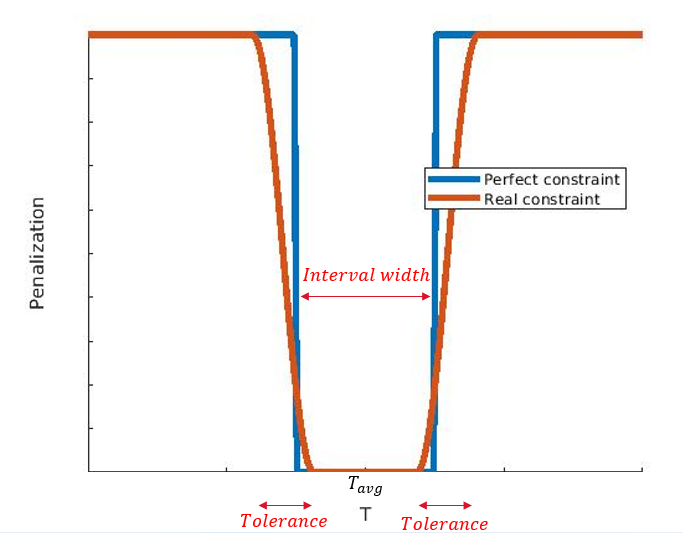
Relaxation of temperature variance penalization

How to interprete the constraint

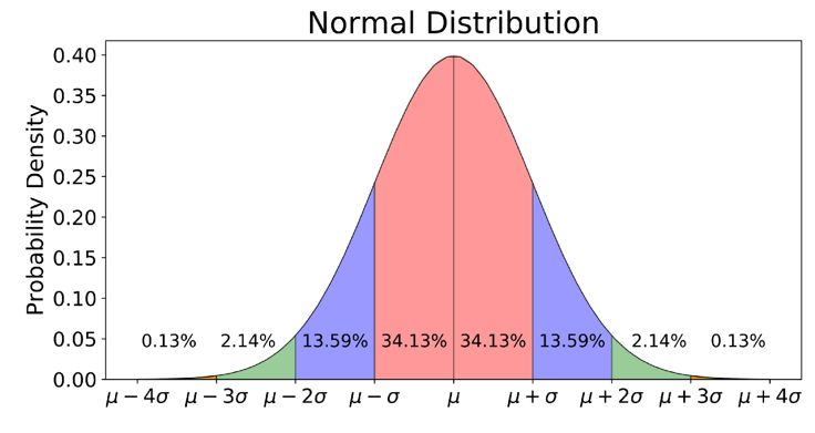
The input parameter for this constraint is the maximum allowed variance. In order to explain how this input value influences the desired temperature interval, we need to go back to the Gaussian curve. We know that 6 times the standard deviation (which equals the square root of the variance) accounts for 99.7% of the full data. This means that six times the square root of the input value is equal to the desired temperature interval.

For example, if you want to have a $5K$ temperature difference on your target surface. Inserting this into what was explained above will give you: $6\cdot\sigma=5𝐾$. Reformulating this equation returns the input value for ColdStream: $\sigma^2=\left(\frac56\right)^2=0.6944K^2$.

❗️Important

Constraint: temperature variance: $\sigma^2=x[K^2]$

$\Rarr \Delta T_{99.7\%}=6\sqrt{x}\;[K]$

Gaussian curve

---

VelocityVariance

Name	VelocityVariance
Goal	The velocity variance on a boundary has to be within a certain limit.
Applicable to	Region	Fluid
	Subregion	Not applicable to any subregion types
	Boundary	PressureInlet PressureOutlet
Target input parameter	$\sigma^2_{U,max}$ in $\left[\frac{m^2}{s^2}\right]$: The maximum variance allowable.

Use this constraint when you want the velocity differences across a boundary to be within a certain value. Meaning, the difference between the velocity at any given point and the mean velocity is limited.

Mathematical formulation

Region/subregion:

$$C = \frac1S\int_S(U-U_{mean})\cdot(U-U_{mean})dS\le\sigma^2_{U,max}$$

Where:

• $C$ is the value of the constraint in $\frac{m^2}{s^2}$.

• $U$ is the velocity distribution on a boundary in $\frac ms$.

• $U_{mean}$ is the mean velocity on the boundary in $\frac ms$.

• $\sigma^2_{U,max}$ is the maximal allowable velocity variance on the boundary in $\frac{m^2}{s^2}$.

• $S$ is the area of the boundary in $m^2$.

Implementation of the constraint on ColdStream

In theory, ColdStream will penalize everything outside of the desired interval width equally. However, the variance constraint needs to be relaxed for two reasons:

• To lower the risk of reaching a local optimum. By relaxing the constraints, ColdStream is far more likely to reach a global optimum.
• To lower the risk of non-convergence.

This relaxation means that near the edges of the desired interval, there are areas where ColdStream does not fully penalize any violations of the constraint. This means that some tolerance will be expected when using this constraint.

	Perfect constraint	Real constraint
Interval width	Exact	Relaxed
Risk local optimum	High	Low
Risk non-convergence	High	Low

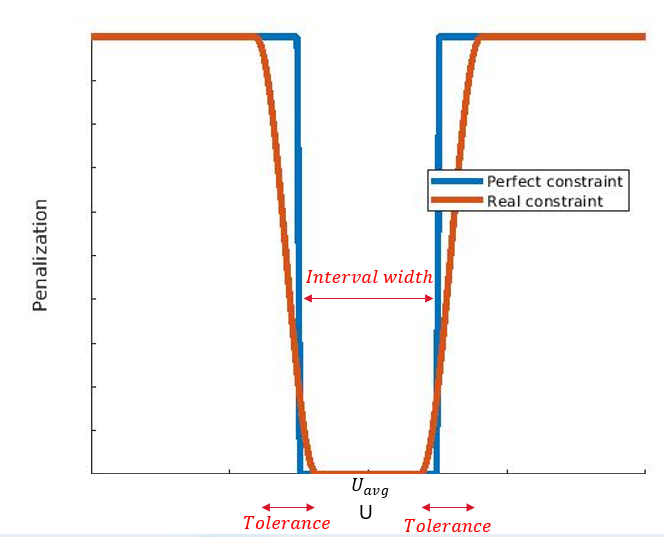
Relaxation of velocity variance penalization

How to interpret the constraint

The input parameter for this constraint is the maximum allowed variance. In order to explain how this input value influences the desired velocity interval, we need to go back to the Gaussian curve. We know that 6 times the standard deviation (which equals the square root of the variance) accounts for 99.7% of the full data. This means that six times the square root of the input value is equal to the desired velocity interval.

For example, if you want to have a $5 \frac ms$ velocity difference on your target surface. Inserting this into what was explained above will give you: $6 \cdot \sigma = 5\frac ms$. Reformulating this equation returns the input value for ColdStream: $\sigma^2=(\frac56)^2 = 0.6944 \frac{m^2}{s^2}$

❗️important

Constraint: velocity variance: $\sigma^2=x[\frac{m^2}{s^2}]$

$\Rarr \Delta U_{99.7\%}=6\sqrt{x}\;[\frac ms]$

Gaussian curve

---

MaximumElectricWirePower

Name	MaximumElectricWirePower
Goal	The design region is used for determining the circuit of an electric wire which heats the region(s) touching the design region. The electric wire power is limited to a certain value.
Applicable to	Region	Not applicable to any region types
	Subregion	Design
	Boundary	Not applicable to any boundary types
Target input parameter	$P_{max}$: The maximal electric power allowable in $[W]$.
Additional input parameters	$V$ in $[V]$: The supplied voltage. $\rho$ in $[\Omega\cdot m]$: Electrical resistivity or the wire.

Use this constraint when the design region is used for determining the circuit of an electric wire which heats the region(s) touching the design region, but has a maximum required electric power. The voltage supplied to the wire circuit and the electrical resistivity of the wire material have to be specified. The result will be an electric circuit with a single wire with a diameter determined by the 'Electric wire' manufacturing specifications. Voltage or frequency control will not be applied, so the wire length will be varied to reach a certain electric power. The design region has to have a constant height. The design region material to be specified is the material of the electrical wire.

Mathematical formulation

$$C=\frac {V^2}{R} = \frac{V^2\pi D^2}{4\rho l}\le P_{max}$$

Where:

• $C$ is the value of the constraint in $W$.

• $P_{max}$ is the maximal electric power in $W$.

• $V$ is the supplied voltage in $V$.

• $R$ is the electrical resistance in $\Omega$.

• $D$ is the wire diameter, taken from manufacturing specifications in $m$.

• $\rho$ is the electrical resistivity of the wire material in $\Omega\cdot m$.

• $l$ is the wire length in $m$.

---

MaximumHeatingTime

Name	MaximumHeatingTime
Goal	Limit the heating time of a region from an initial temperature to a target temperature.
Applicable to	Region	Solid
	Subregion	Not applicable to any subregion types
	Boundary	Not applicable to any boundary types
Target input parameter	$t_{heatup}$: The maximal heatup time in $[s]$.
Additional input parameters	$T_{initial}$ in $[K]$: The initial temperature. $T_{target}$ in $[K]$: The target temperature.

Use this constraint when the heatup time of a region should be limited. The heatup time is the time it takes for the region to heat up from an initial temperature to a target temperature. Note that the target temperature does not have to be the final temperature the region reaches, it can be smaller.

Mathematical formulation

$$C = 5\tau_c=5\cdot\frac{\rho c_pV(T_{initial}-T_{target})}{Q} \le t_{heatup}$$

Where:

• $C$ is the value of the constraint in $s$.

• $t_{heatup}$ is the maximal heatup time in $s$.

• $\tau_c$ is the time constant in $s$.

• $Q$ is the heat supplied to the region in $W$.

• $\rho$ is the density of the region in $W$.

• $c_p$ is the heat capacity of the region material in $\frac{J}{kg\cdot K}$.

• $V$ is the volume of the region in $m^3$.

• $T_{initial}$ is the initial temperature of the design region in $K$.

• $T_{target}$ is the target temperature of the region in $K$.

---

Weighting functions

Introduction

When using the Diabatix platform, one can assign multiple targets when setting up a design case. One can choose both multiple objectives and constraints. When selecting multiple objectives, this is technically a multi-objective optimization, and the importance of each objective can be changed relative to each other. When selecting multiple constraints, each constraint will be satisfied as long as they are physically possible. The satisfaction of constraint(s) will always take priority over minimizing/maximizing objectives.
A weighting value allows the user to specify the importance of each objective. After selecting a desired objective, you can change the weighting factor of it.
A weighting value equal to 1 translates to that objective having the highest priority, while a value close to 0 translates to the target having the lowest priority.

📘

Note

Multiple objectives can have the same weighting factor. For example, two objectives can both have a weighting factor equal to one. This translates to both objectives being equally important and for this example, both objectives have the highest priority.

The concept of a Pareto front is very important when doing multi-objective optimization and will be discussed in the following section. The next section explains how weighting factors imposed on objectives influence the optimal design. The final section explains how weighting factors imposed on constraints impact this optimal design.

👍

Example

To make this article easier to understand, a simple thermal optimization problem will be used. This simple thermal problem only has 2 objectives, a temperature objective and a pressure objective.

Pareto front

"Many real-world optimization problems presume a vector of conflicting objectives. These objectives are to be optimized simultaneously" [1]. "The optimal solution of a multi-objective problem is not unique, instead there exists a Pareto optimal solution set. For a specific optimization problem, a final compromised solution should be specified from the Pareto optimal solution set according to the preference of the designer or the actual demand" [2].

This compromised solution can be selected in two manners:

1. changing the weighting factors of each of the objectives and/or
2. by imposing constraints.

The Pareto front represents all optimal solutions where if one target is improved, at least one other target must deteriorate for the problem to remain feasible. This condition is what is known as a Pareto optimal solution. Everything above the Pareto front is a feasible solution, but sub-optimal. Everything below it is infeasible.

👍

Example

For our simple thermal problem this will translate to the following: For any optimal design will there be another one that can reduce the temperature further at the cost of an increased pressure drop?
For instance, the other design has narrower channels which aids the heat transfer to/from the fluid, but this will increase the pressure drop when the fluid flows through it.

📘

Note

Two objectives with the same name (e.g. temperature minimization) are treated separately. The weighting factors are not summed!

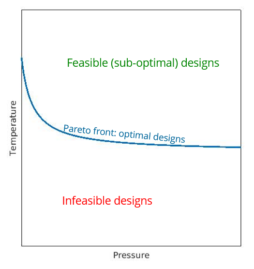
Pareto front

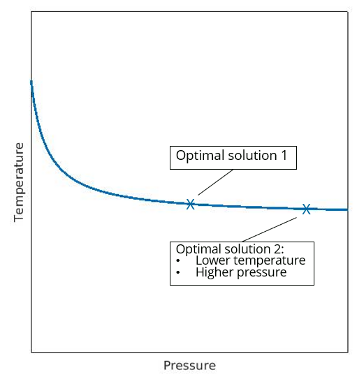
Pareto front: 2 Pareto optimal solutions

Weighting factors for objectives

As stated in the introduction, giving a higher weighting factor to an objective translates to that objective having a higher importance. The difficulty with doing an optimization based solely on objectives is the fact that it is a priori uncertain what design on the Pareto front will be returned. It only allows us to put all objectives in a hierarchy.

A constraint, on the other hand, allows one to more easily specify which point on the Pareto front is the desired one (more on this in the next section).

👍

Example

For our simple two-objective problem: if you assign a higher weighting factor to the temperature minimization objective compared to the pressure minimization objective, the generative design tool will return a design that favors a reduction in temperature over a reduction in pressure. Switching the weighting factors of the objectives will result in the generative design tool returning a design favoring a lower pressure drop over a lower maximum temperature.

❗️

Important

Only using objectives will not give you great control over the Pareto optimal solution.

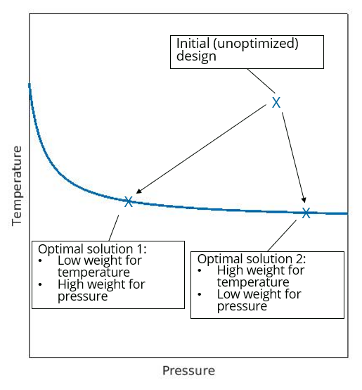
Influence of weighting factors for pure multi-objective optimization

Weighting factors for constraints

Constraints are targets that must be satisfied at all times. Meaning that they are more restrictive to the final (optimal) design compared to objectives. Due to this definition, prioritizing constraints through weighting factors is irrelevant.

Constraints are inherently more powerful than objectives and are thus capable of decreasing the size of the Pareto optimal solution set. However, one must be careful when assigning them. Setting too many constraints or setting constraints that are too strict can make the optimization problem infeasible (the Pareto optimal solution set is empty). Running a simulation (called a control simulation) before doing a design will help you understand the problem (and its potential limits). This in turn will allow you to select more feasible constraints.

The support engineers at Diabatix can also help you with setting up a feasible design case as this group has a lot of experience with multi-objective optimization problems.

👍

Example

Going back to our simple thermal problem one last time. If the control simulation shows that the maximum temperature of the geometry is 60°C and the pressure drop through it is 20kPa. The problem will most definitely become infeasible when setting a maximum temperature constraint equal to 10°C and minimizing the pressure drop.

❗️

Important

Constraints allow greater control over which Pareto optimal solution will be returned. However, the problem can become infeasible!

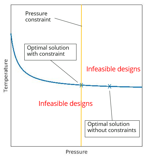
Influence of constraint on feasible solutions

References

1. Jyotsna K. Mandal, Somnath Mukhopadhyay, and Paramartha Dutta. multi-objective Optimization. Springer Singapore, 2018
2. Xu Han and Jie Liu. Introduction to multi-objective Optimization Design. eng. In: Numerical Simulation-based Design. Singapore: Springer Singapore, 2020, pp. 141-151. ISBN:9789811030895.