Case type

Introduction

ColdStream supports 4 types of cases. The type of case dictates what ColdStream needs to do. Here you find a summary of all supported case types:

1. Base case
2. Simulation
3. Custom design
4. Standard design

As highlighted in this article, to successfully design a heatsink, we strongly advise to follow a workflow. A workflow is a combination of cases. A workflow always starts with a base case. This type of case cannot run but contains the initial geometry and input.

Secondly, ColdStream supports regular CFD simulations. These can be set up for cases of type 'simulation'. Simulations are ideal early on in the workflow or to validate one or more designs later on in the workflow.

Lastly, ColdStream offers two different forms of generative design, where ColdStream will generate designs based on user-specified targets. The difference between standard designs and custom designs will become clear in their dedicated chapters. The generative design cases rely on CFD simulations during the design process, hence why the third option is explained first.

Base case

The base case serves as the foundation for the rest of the workflow. This case contains the initial geometry and input parameters upon which all subsequent cases will be built. It represents an initial configuration or scenario that can be modified and optimized to meet specific requirements. It is recommended for engineers to start with the base case to analyze its performance and identify areas for improvement.

---

Simulation

Introduction

This chapter describes the modeling approach used within ColdStream to perform CFD simulations. The equations used to model the fluid and solid regions' physical behavior are explained. The different turbulence models, used to describe the turbulent behavior of fluids, available in ColdStream are also described.

Fluid region

Navier-Strokes equations

In ColdStream, the physical behavior of fluids is modeled using the Navier-Stokes equations, conservation of mass and momentum, in combination with the energy equation. [1], [2]
For incompressible fluids, the continuity equation can be written as:

$$\frac{\partial\rho}{\partial t} + \nabla \cdot \rho \vec v = \rho \nabla \cdot \vec v = 0$$

Where $\rho$ represents the density field, $\vec v$ is the velocity field and $t$ is the time.

The incompressible flow assumption holds well for all fluids at low Mach numbers (up to approximately 0.3). For higher Mach numbers, the compressibility effects cannot be ignored and should be taken into account. The Mach number for gas flows can be calculated using the following equation (liquids are always assumed to be incompressible):

$$M = \frac{v}{c}=\frac{v}{\sqrt{\gamma RT}}$$

Where $v$ is the velocity magnitude, $c$ represents the speed of sound, $\gamma$ is the heat capacity ratio, $R$ is the specific gas constant and $T$ is the temperature.

The conservation of momentum can be written as:

$$\rho \frac{\partial \vec v}{\partial t} + \rho \vec v \cdot \nabla \vec v = - \nabla \rho + \nabla \cdot \mu \nabla \vec v + \vec f$$

Where $\vec v$ is the velocity field, $\rho$ is the density, $\mu$ is the dynamic viscosity, $p$ is the pressure and $\vec f$ an optional body force (for example gravity).

The energy equation, as a function of enthalpy, can be written as:

$$\rho \frac{\partial \vec v}{\partial t} + \rho \vec v \cdot \nabla h - \rho \nabla \cdot \alpha \nabla h = Q$$

Where $\alpha$ is the thermal diffusivity and $Q$ is an energy source (for example an internal heat source due to an exothermic reaction).

The thermal diffusivity is defined as:

$$\alpha = \frac{k}{\rho c_p}$$

Where $k$ represents the thermal conductivity and $c_p$ the specific heat capacity.

The following equation relates the enthalpy to the temperature for incompressible fluids:

$$dh=c_pdT$$

The energy equation can therefore be easily written in terms of the temperature:

$$\rho c_p \frac{\partial T}{\partial t} + \rho c_p \vec v \cdot \nabla T - \nabla \cdot k \nabla T = Q$$

Body forces

For forced convection applications:

$$\vec f = \vec 0$$

For natural convection applications, the body Boussinesq approximation is applied to model the buoyant behavior of the fluid. Therefore, the body force is taken as:

$$\vec f = \rho (1- \beta (T-T_{ref}))\vec g$$

Where $\vec g$ is the gravitational acceleration, $\beta$ the coeficient of expansion. Note that $\beta$ is taken as a function of the reference temperature $\left( T_{ref} \right)$ and therefore is constant during the simulation.

Turbulence model

Different modeling approaches exist to predict the effects of turbulence on a flowing fluid. An overview of the available turbulence models within ColdStream and a flow chart to help you select the best model for your specific problem can be found here.

Solid region

For the solid region, only the energy equation needs to be solved:

$$\rho \frac{\partial h}{\partial t} - \rho \nabla \cdot \alpha \nabla h = Q$$

Where $\rho$ is the density of the solid material, $h$ is the enthalpy, $\alpha$ represents the thermal diffusivity and $Q$ is a heat source (for example due to Joule heating).

Similarly to the fluid equations, the solid energy equation can also be written in terms of the temperature:

$$\rho c_p \frac{\partial T}{\partial t}-\nabla \cdot k \nabla T = Q$$

Where $c_p$ is the specific heat capacity and $k$ represents the thermal conductivity of the solid material.

ColdStream allows the use of either isotropic or anisotropic properties, depending on the material thermophysical properties.

Interface modeling

The heat exchange between different components, for example, a solid and a fluid, depends only on the temperature difference between the respective cells adjacent to the wall. At this wall, interface equilibrium conditions are imposed, requiring that the heat flux over the interface is equal and from the fluid side only dependent on the effective thermal conductivity, which accounts for the thermal conductivity of the fluid and the turbulent diffusivity:

$$k_{solid} \nabla T_{solid} = k_{fluid} \nabla T_{fluid}$$

Furthermore, the temperature on each side of the interface between a fluid and a solid should match:

$$T_{solid}=T_{fluid}$$

While computationally expensive, this approach provides a detailed insight into the physics of the problem, which in turn, will provide the optimizer with a more realistic performance of each design. This is fundamental to correctly exploring the design space and eventually finding a truly optimal design.

References

1. https://www.eng.auburn.edu/~tplacek/courses/fluidsreview-1.pdf
2. https://www.grc.nasa.gov/www/k-12/airplane/nseqs.html

---

Standard design

Introduction

The standard design selector is an efficient and effective way to generate standard heatsink designs that are widely available on the market. A few examples are fin heatsinks for LEDs, extruded heatsinks for PCBs, heatsinks for processors, etc.

Standard fin heatsink example with a fan on top of it

📘

Note

Standard design cases optimize for the best off-the-shelf heatsink for your case.

A heatsink transfers heat from a component to a fluid medium where the heat is dissipated away. The general idea is the more surface area there is, the better the heatsink will perform.

Off-the-shelf heatsink options

As a ColdStream user, you have full control over what shapes ColdStream needs to consider as well as the manufacturing settings to make those structures.

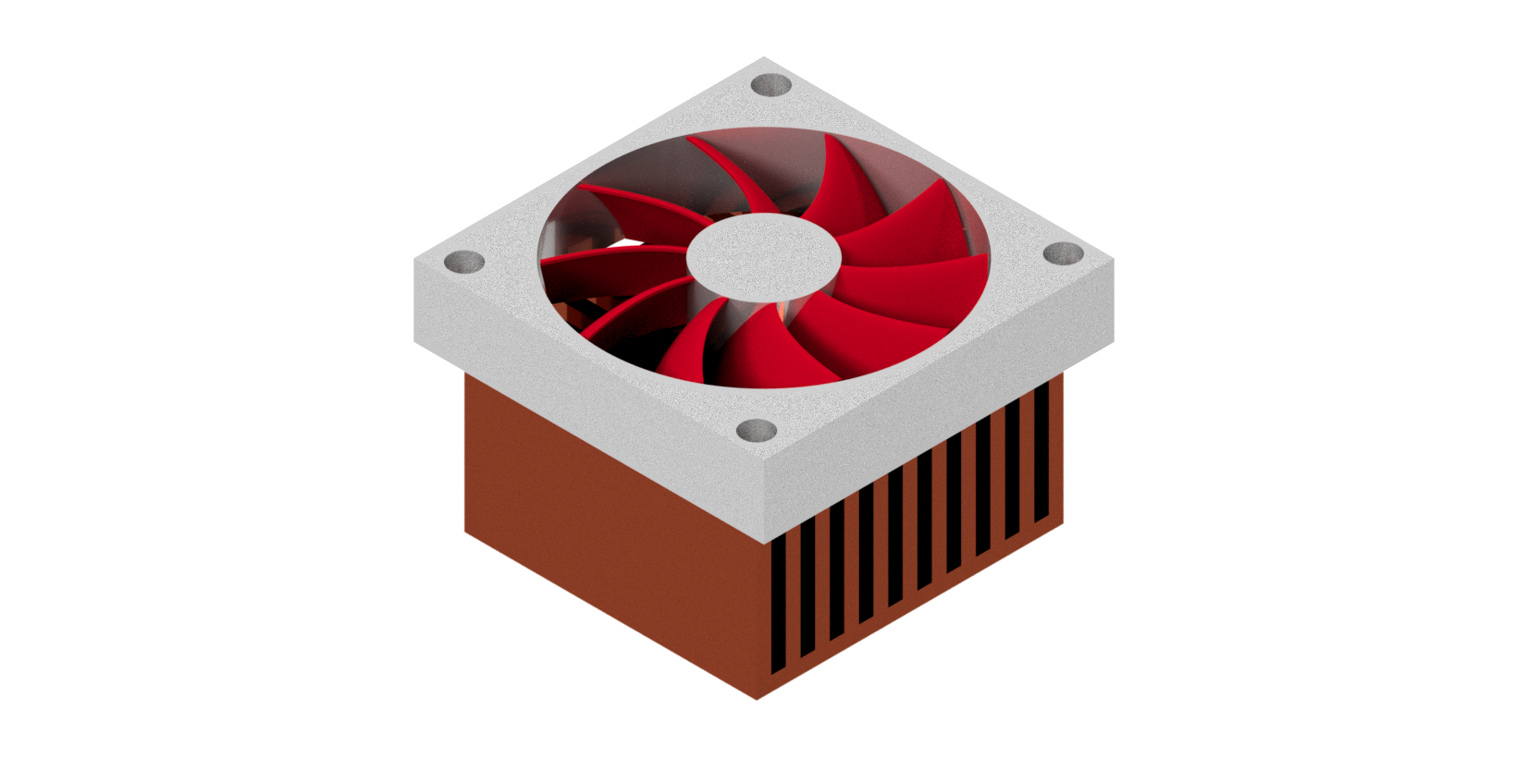
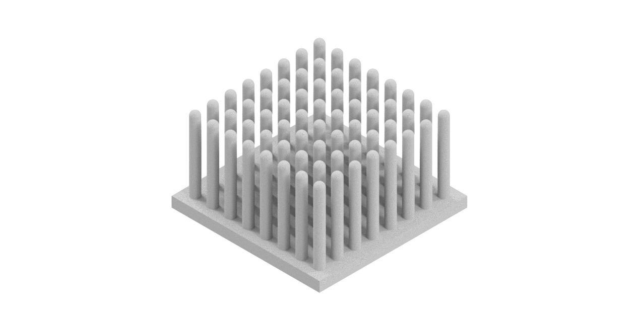
Pins and fins

As the name already indicates, a pin heatsink has pins extruding from its base plate. These pins can have circular, rectangular, or diamond-shaped cross-sections. As a user, you have control over which options ColdStream can consider.

A pin heatsink is one of the most common heatsink types on the market. Pin heatsinks have a large surface area given the heatsink volume, which makes them perform well for any possible orientation. For pins heatsinks, the growth of the thermal boundary layer along the direction of the airflow is limited by the discontinuous surface formed by the pins. In addition, the discontinuous geometry of the pins also increases the pressure drop across the heatsink which causes a lower flow rate for a given in- and outlet pressure condition.

Example of a pin heatsink

For a finned heatsink, the design is not discontinuous anymore in 1 of the 2 horizontal directions. This will cause the thermal boundary layer to build along the entire surface of the fin.

Example of a fin heatsink

📘

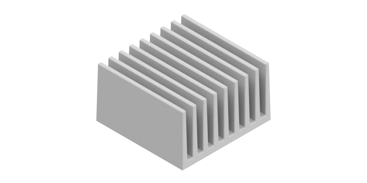
Note

Research has shown that fin heatsinks perform better for most of the natural convection cases.
Pins are advantageous when the incoming fluid flow can come from multiple directions as the performance is more or less independent of the orientation. Fins perform poorly when the fluid flow is perpendicular to it.
In forced convection cases, research has shown pin heatsinks to outperform fin heatsinks even when considering the increased pressure drop across the pins.

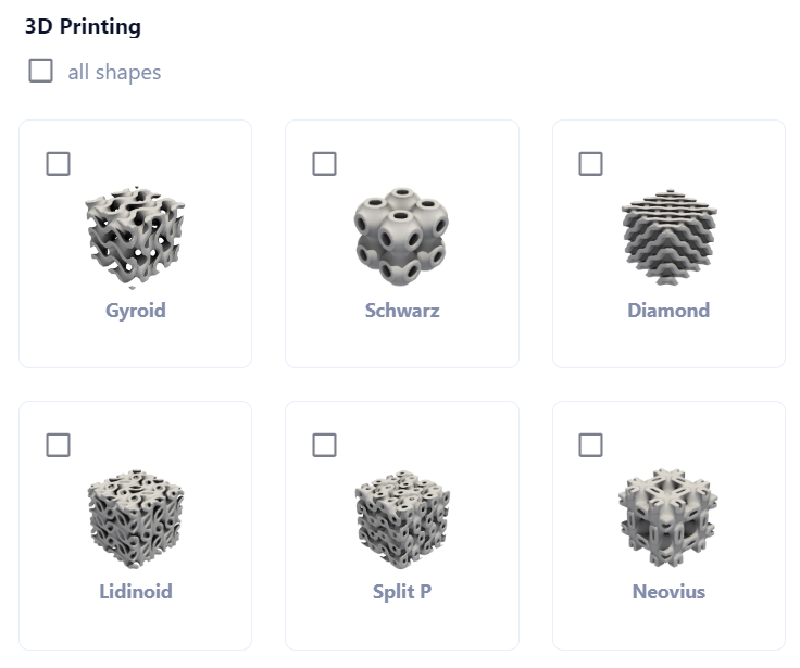
3D printed TPMS structures

With the boom in popularity of additive manufacturing techniques, like SLS, SLM, and LPBF, more complex shapes can now also be considered for heatsinks. As a ColdStream user, you have now the option to optimize for the following Triply Periodic Minimal Surfaces (TPMS) structures:

• Gyroids
• Schwarz
• Diamond
• Lidinoid
• Split P
• Neovius

Available TPMS structures

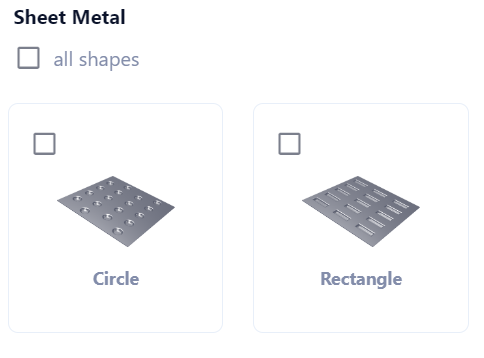
Sheet metal formed dimples

Sheet metal forming is a cheap manufacturing process for large volumes. It also results in light designs. This makes it very attractive in the automotive industry, mainly for battery cold plates. The off-the-shelf designs available for this manufacturing technique are circular and rectangular dimples.

Available dimples

Case setup

There are only 2 differences between the setup of a standard design case and regular CFD simulation. The first difference is that the CAD file doesn't contain any cooling structures, this has been replaced with a design domain. The design domain is the volume where ColdStream is allowed to generate these off-the-shelf heatsinks. Secondly, targets are needed to let ColdStream know what to optimize for.

For standard designs, the design region should be oriented along the Cartesian axes. The design region can take arbitrary shapes, but it is advised to have a flat base.

❗️

Important

The design region should be oriented along the Cartesian axes. The parent region of the design should be of type fluid and at least one of the flat faces of the design region should touch another region of type solid.

Example design subregion

❗️

Important

The design subregion must be able to accommodate at least 5 fins/pins in each direction. The minimal width of the pins/fins equals 1 mm.

ColdStream will also generate a baseplate with a thickness of at least R_f,min.

The user has the option to select one or more of these manufacturing options according to the user's manufacturing capabilities. The results will contain the best heatsink for each manufacturing type from which the user has the option to select the one that suits them the best. It is also possible to select multiple materials for the heatsink. However, Diabatix advises to limit the number of design variables as much as possible and split it up over multiple cases.

📘

Note

As a user, you can select multiple shapes and/or manufacturing settings and/or materials withing one standard design case. However, Diabatix advises to limit the number of design variables at much as possible by splitting it up into multiple standard design cases. For example, consider CNC milled pins in one case, and 3D printed Gyroids in another.

The correlation based standard design mode allows you to very quickly gain insights into what works best for your case using minimal resources.

Once the case setup is complete, you are ready to validate the case setup and submit the case. After the submission, the optimizer iterates through several pre-defined parameters of a heatsink and optimizes them. The parameters include, but are not limited to the element (pin or fin) dimensions, the base plate dimensions, and the number of elements. The results of a standard design will also show the parameter set that defines a particular heatsink.

Results

The results show a detailed evolution of the optimization. For each design iteration, the geometry, performance, and multiple contours of fields are available on the platform. The design evolution is plotted with the design iteration on the x-axis and the performance of that design on the y-axis. You can access the parameters of the heatsink for a particular design iteration and choose to view the results for that iteration.

---

Custom design

Introduction

Custom design is another form of generative design, where ColdStream has complete flexibility to generate a custom heatsink solution. Compared to standard designs, ColdStream is not limited anymore to off-the-shelf heatsinks.

As a user, you can constrain what structures ColdStream can return by specifying a manufacturing technique and its governing settings. For more information about the available manufacturing techniques and settings, please have a look at this article.

Example result of a custom design case using CNC milling. Where the green volumes are the milled structures

Case setup

The case setup of a custom design is almost identical to the one of a standard design case. The CAD geometry is again of an empty design, where the design domain dictates what volume can be used by ColdStream to generate the heatsink structures. The differences with a standard design case are:

1. The design domain doesn't need to be aligned with the Cartesian axes.
2. The parent region can be a solid, it mustn't be a fluid
3. The design region can touch another solid body, but it is not required
4. No baseplate is being generated

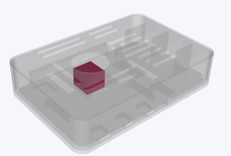
Initialization

As a user, you have some control over the outcome of a custom design case. By initializing the design domain with your design or a previous design from ColdStream, you can push ColdStream in the desired direction. To benefit from initialization, please follow these steps:

1. You navigate to the design domain of interest and turn the initialization slider on.
2. Next, you upload a STEP or STL of the initial design. Do know that only the parts that overlap with the design domain will be taken into account for the custom design.
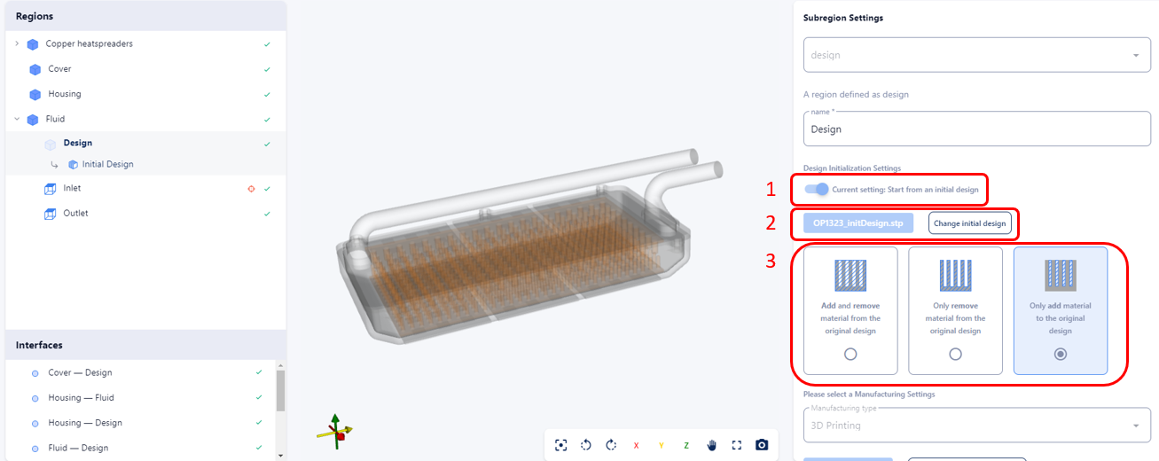
3. Finally, you let ColdStream know what type of initialization you would like to use. ColdStream supports 3:
   1. Only add: the initial design is untouched, ColdStream can only add material in between the channels.
   2. Only remove: the channels of the initial design are untouched, ColdSteam can only take away material from the initial design.
   3. Add and remove: this is a pure initialization, ColdStream is free to add structures around your initial design as well as remove material from it.

Initialization in ColdStream

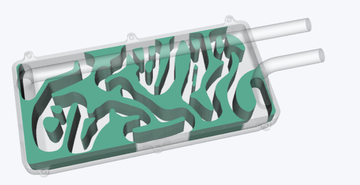
Results

The results show a detailed evolution of the optimization. ColdStream will output a handful of data points. For each data point the geometry, performance, and multiple contours of fields are available on the platform. The design evolution is plotted with the design iteration on the x-axis and the performance of that design on the y-axis. You can access the parameters of the heatsink for a particular design iteration and choose to view the results for that iteration.